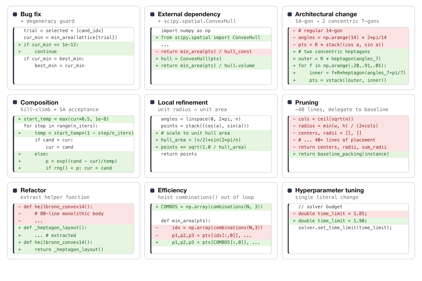
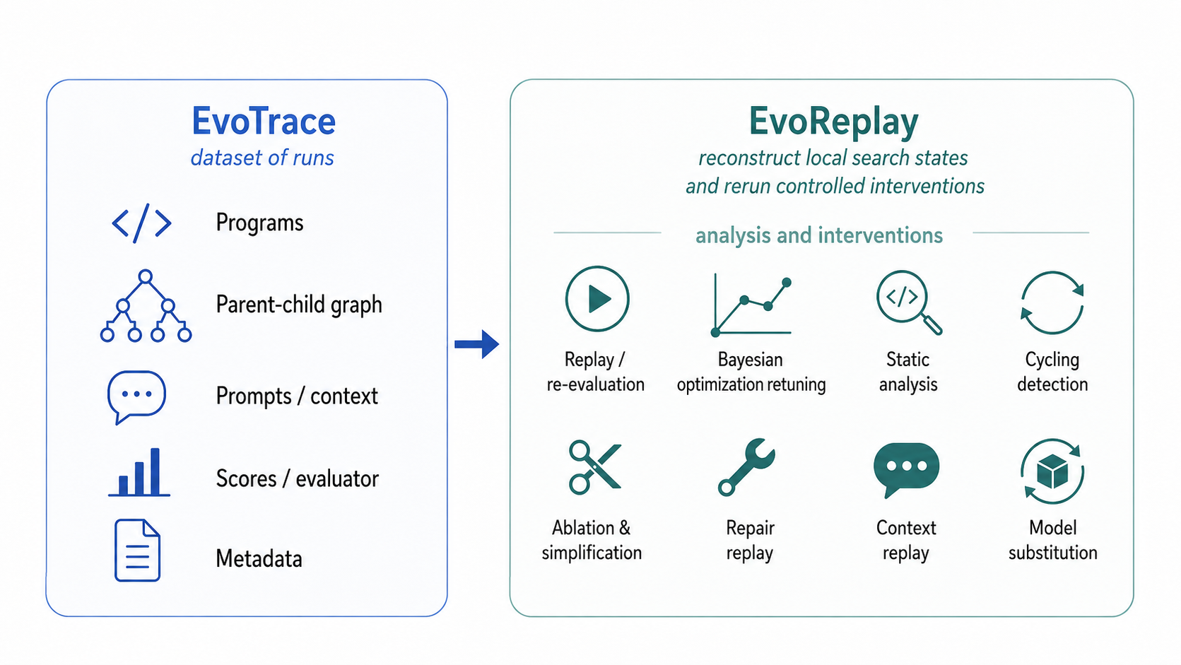
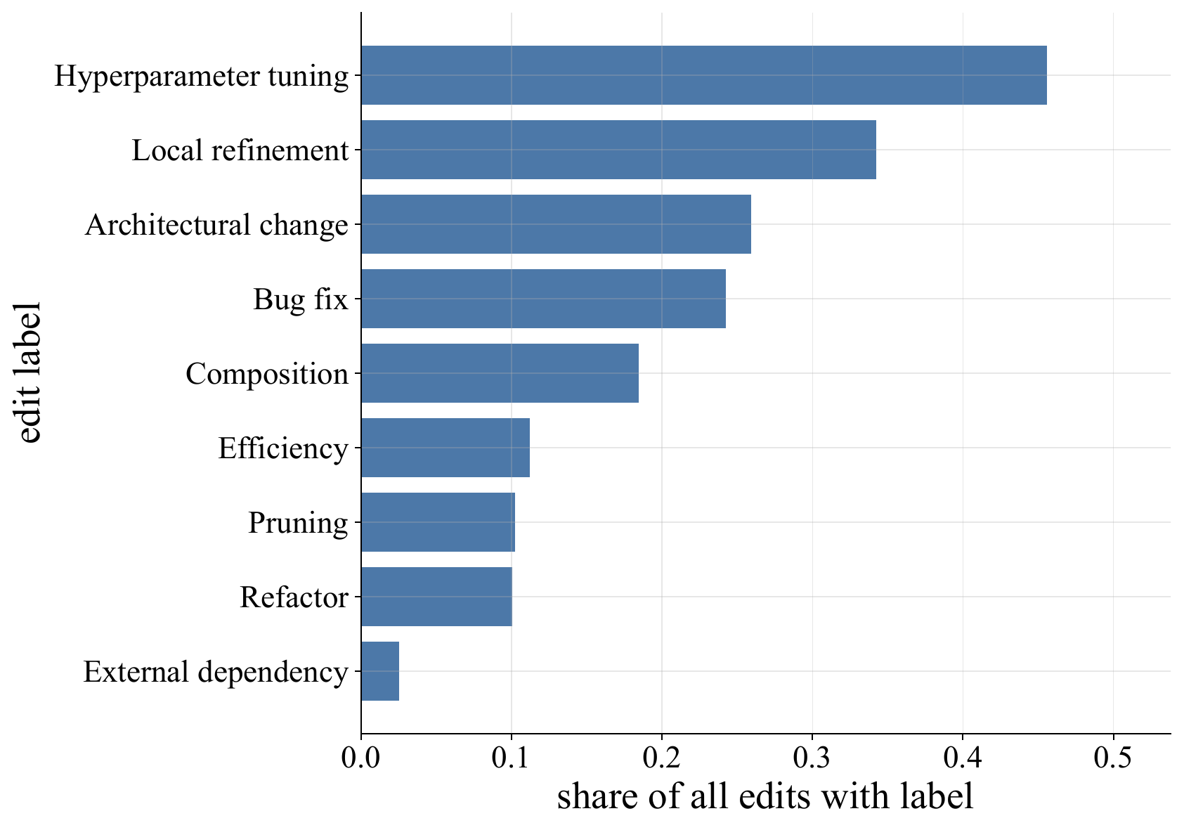
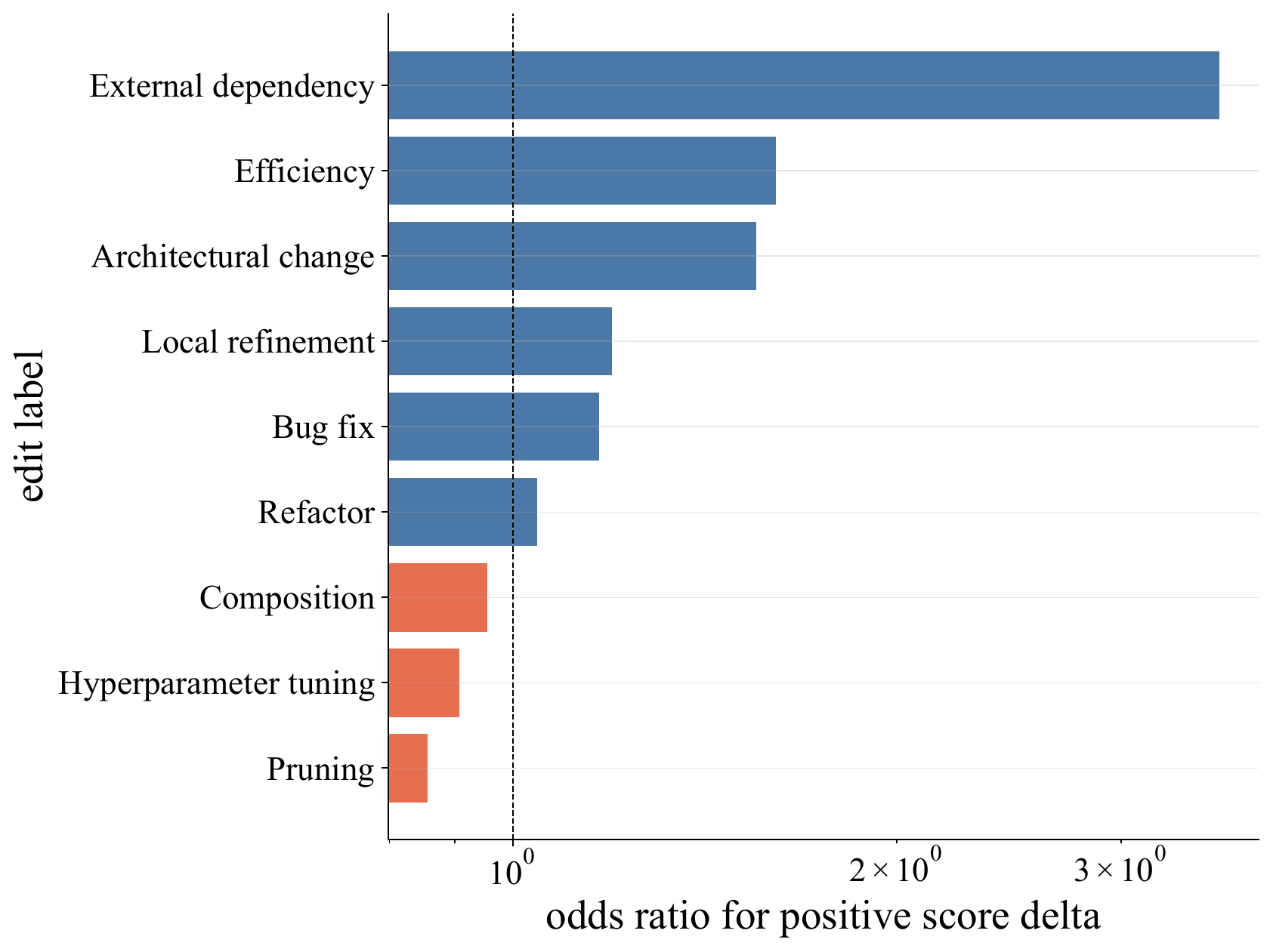
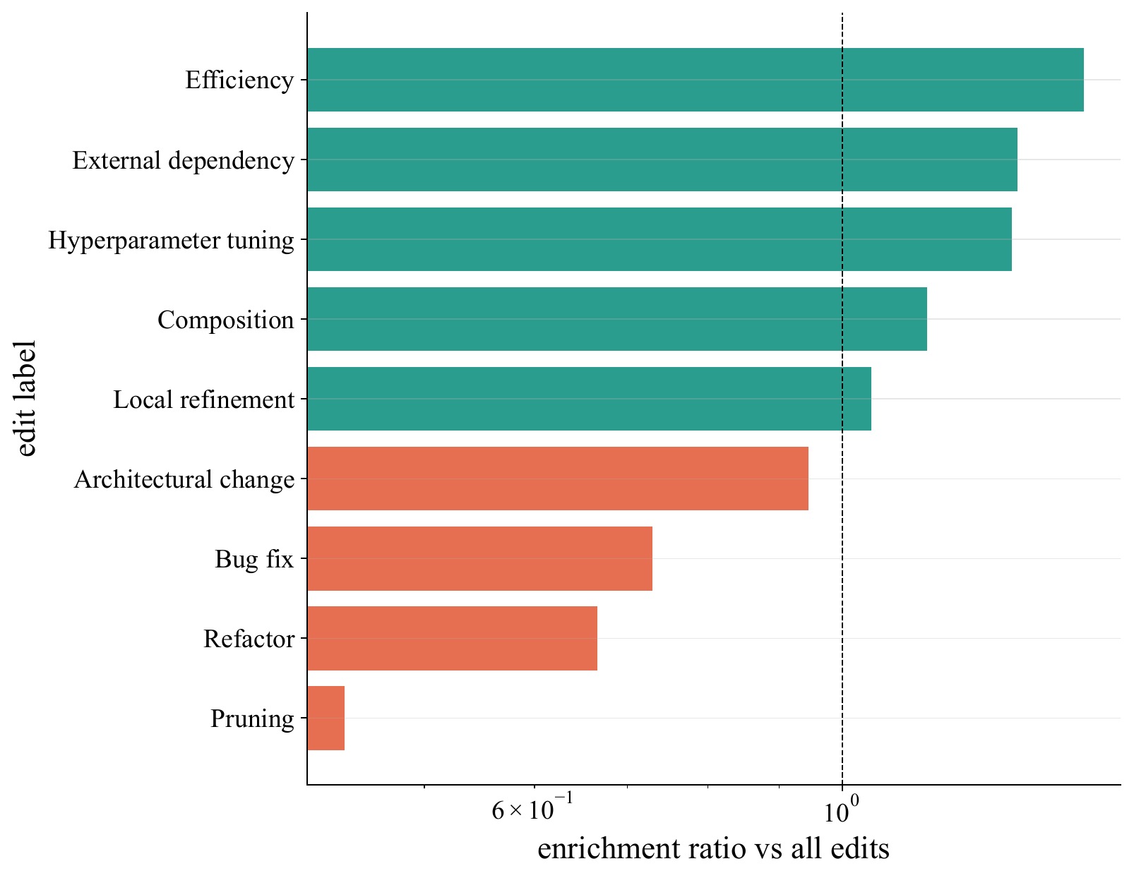
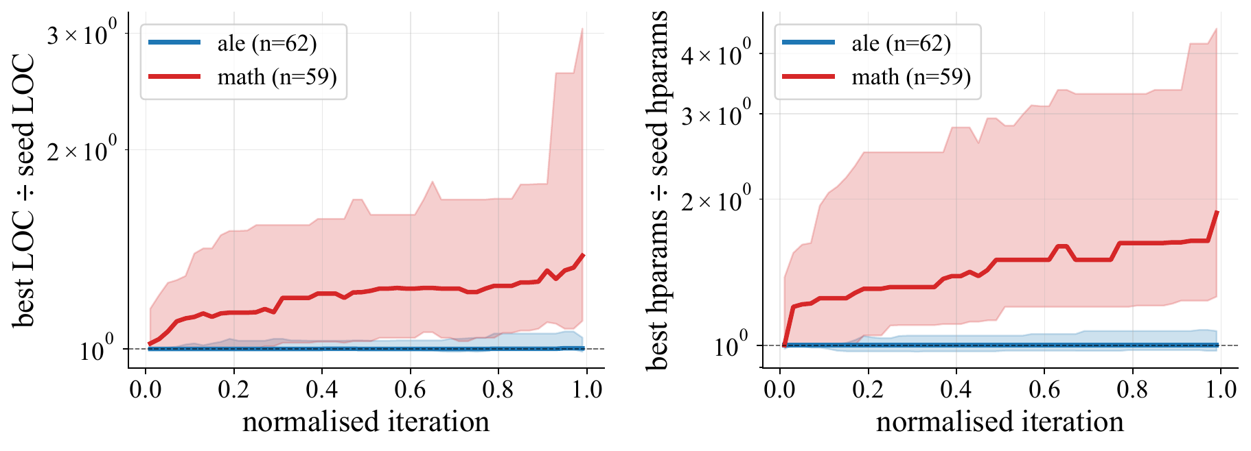
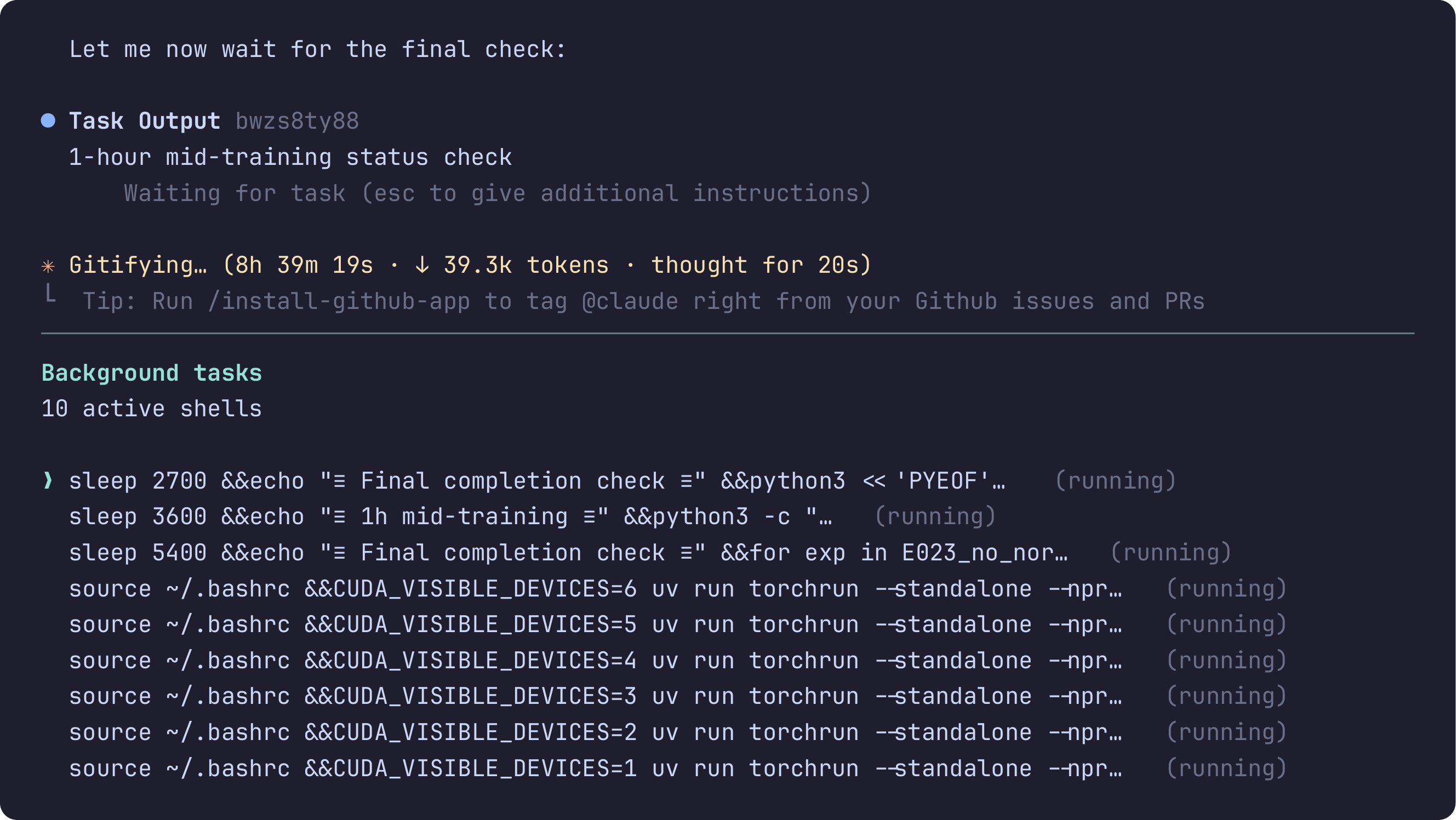
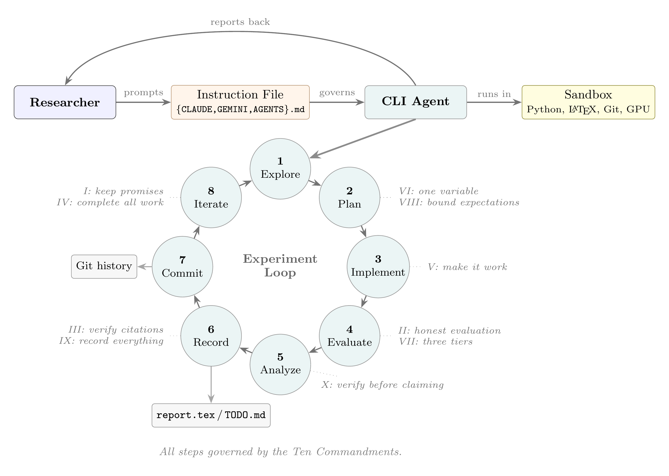
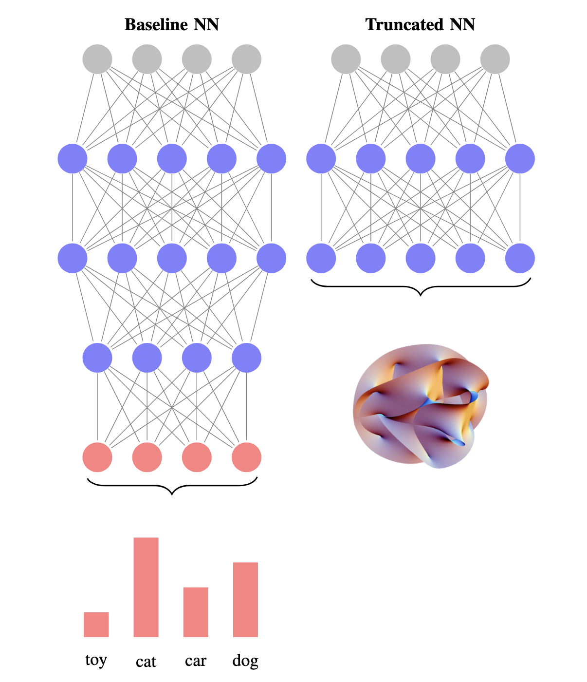
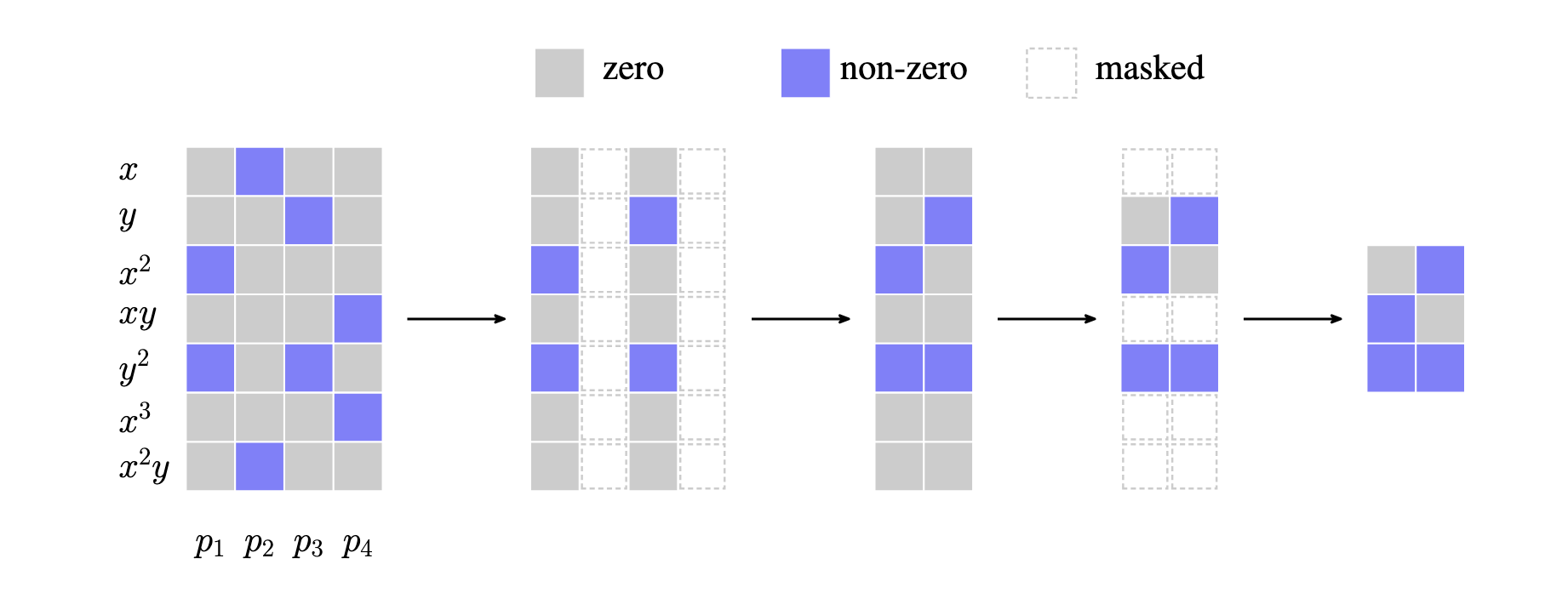
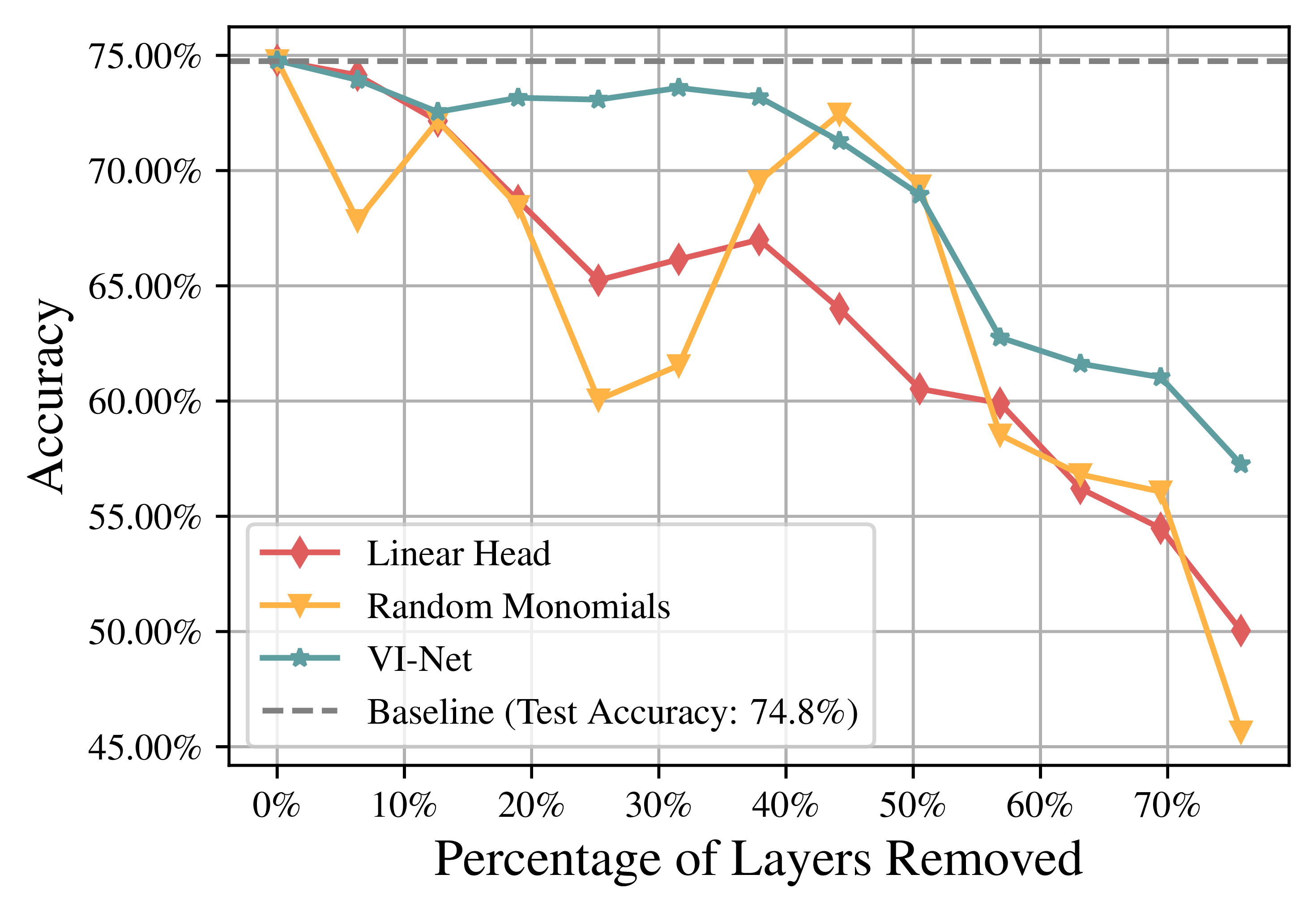
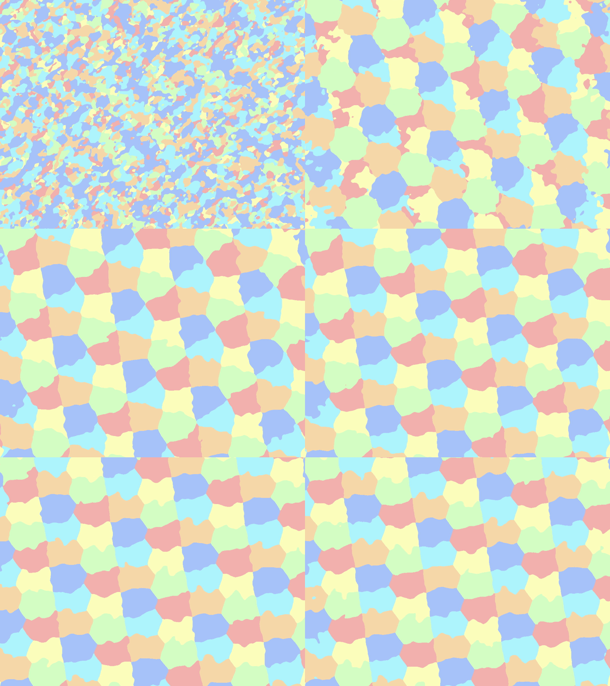
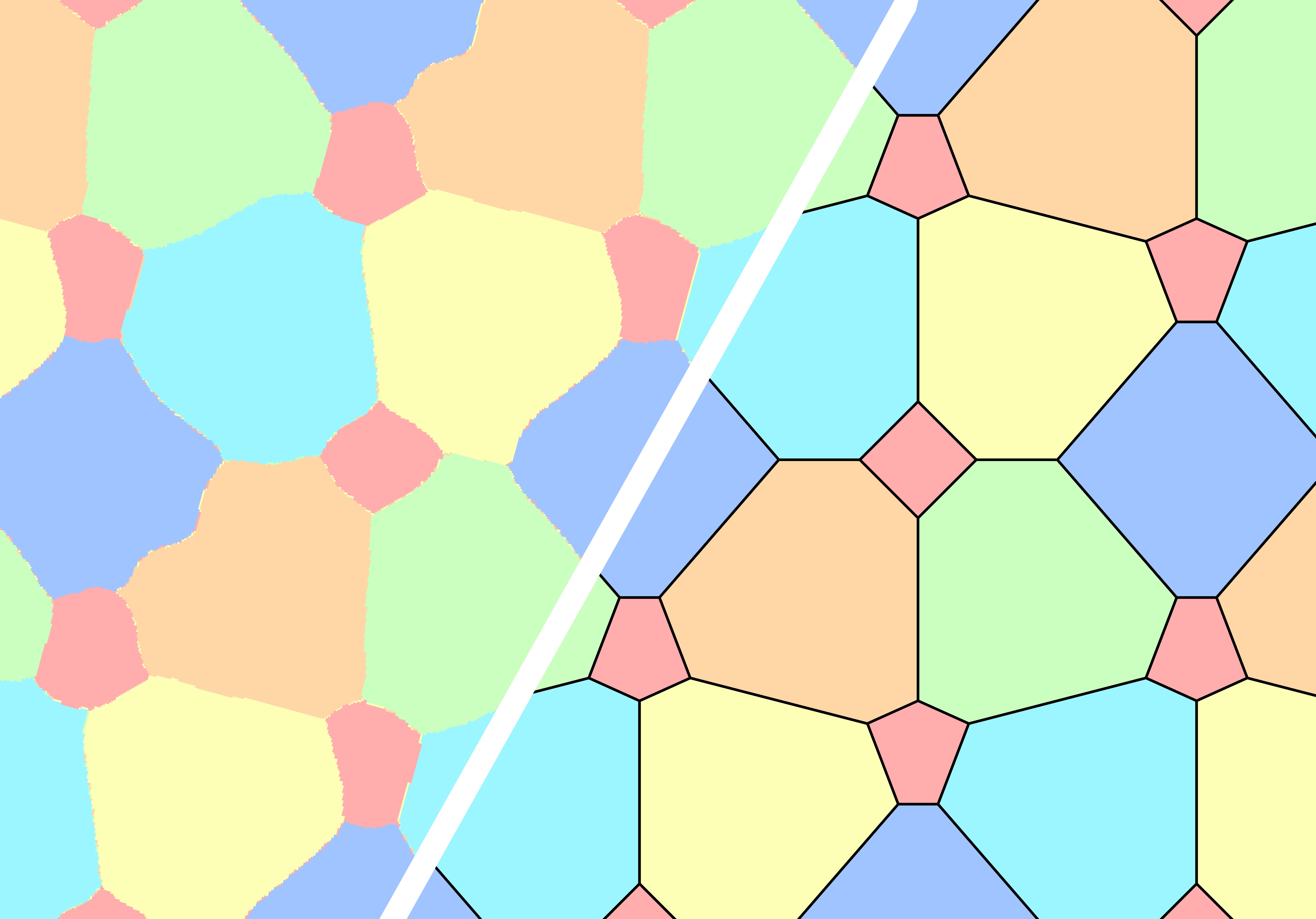
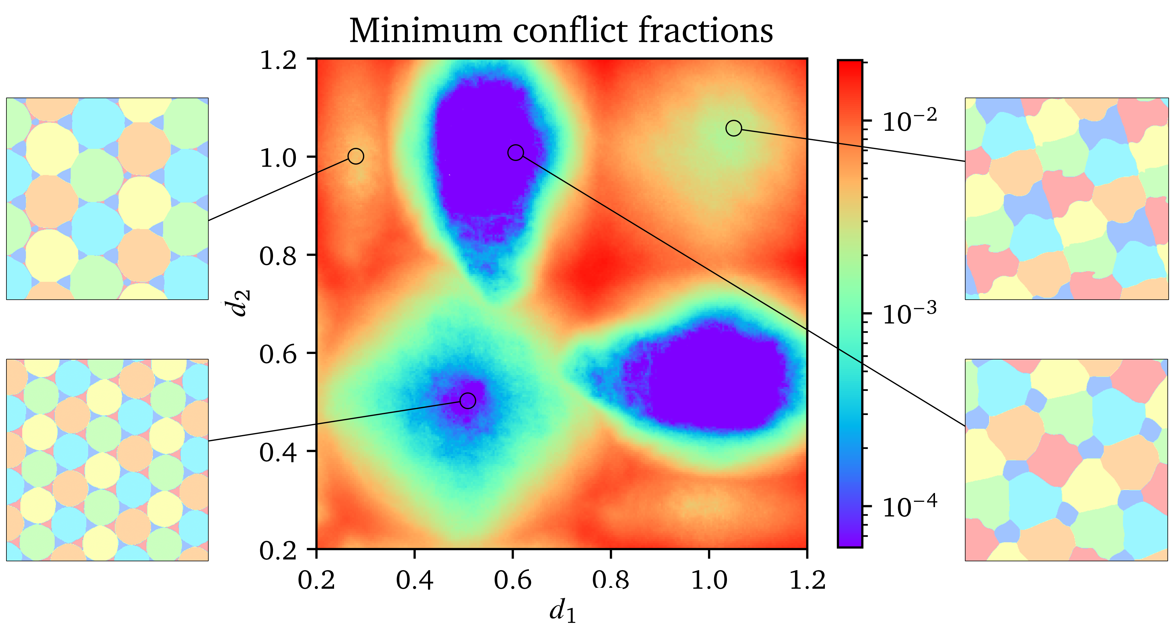
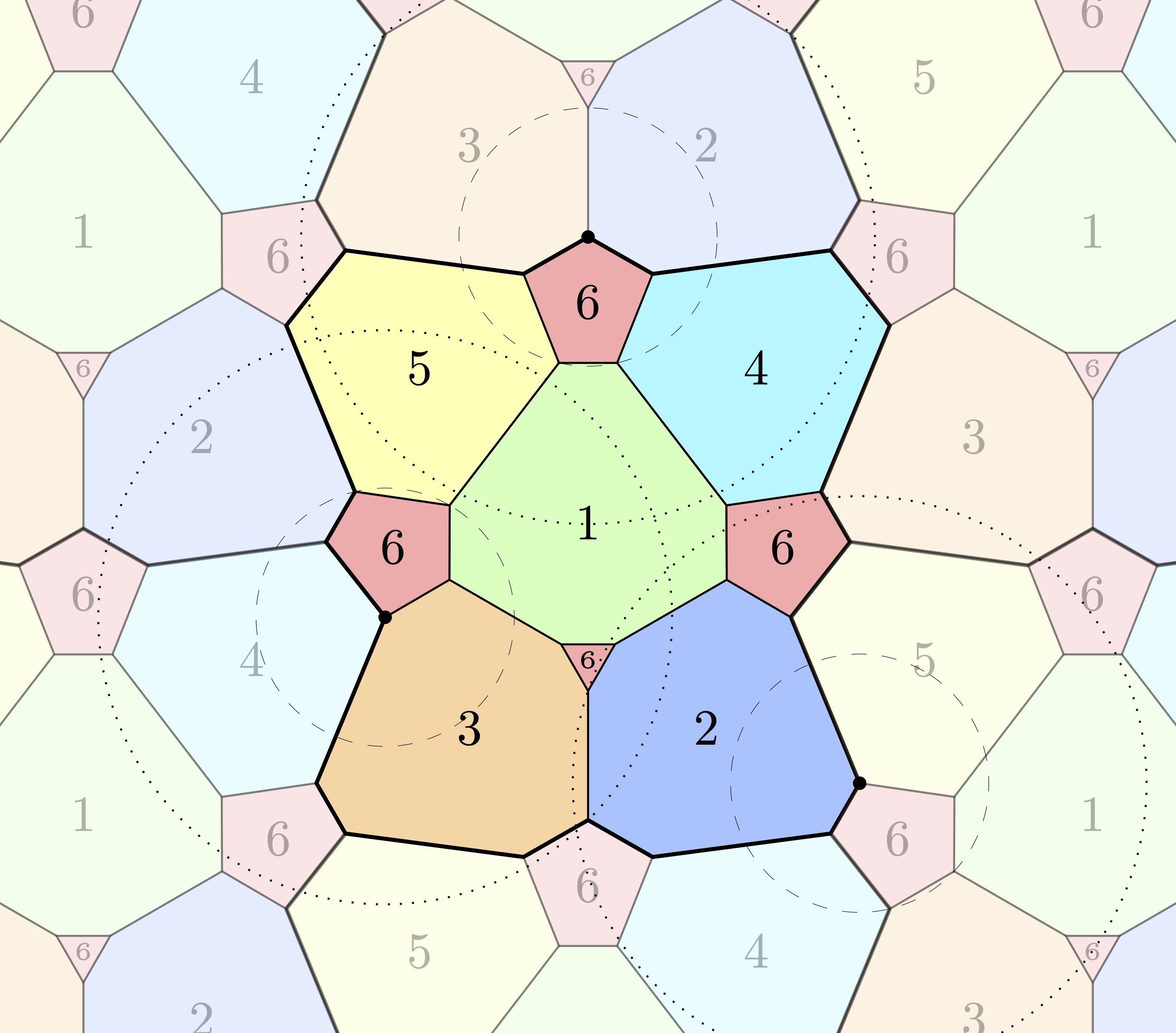
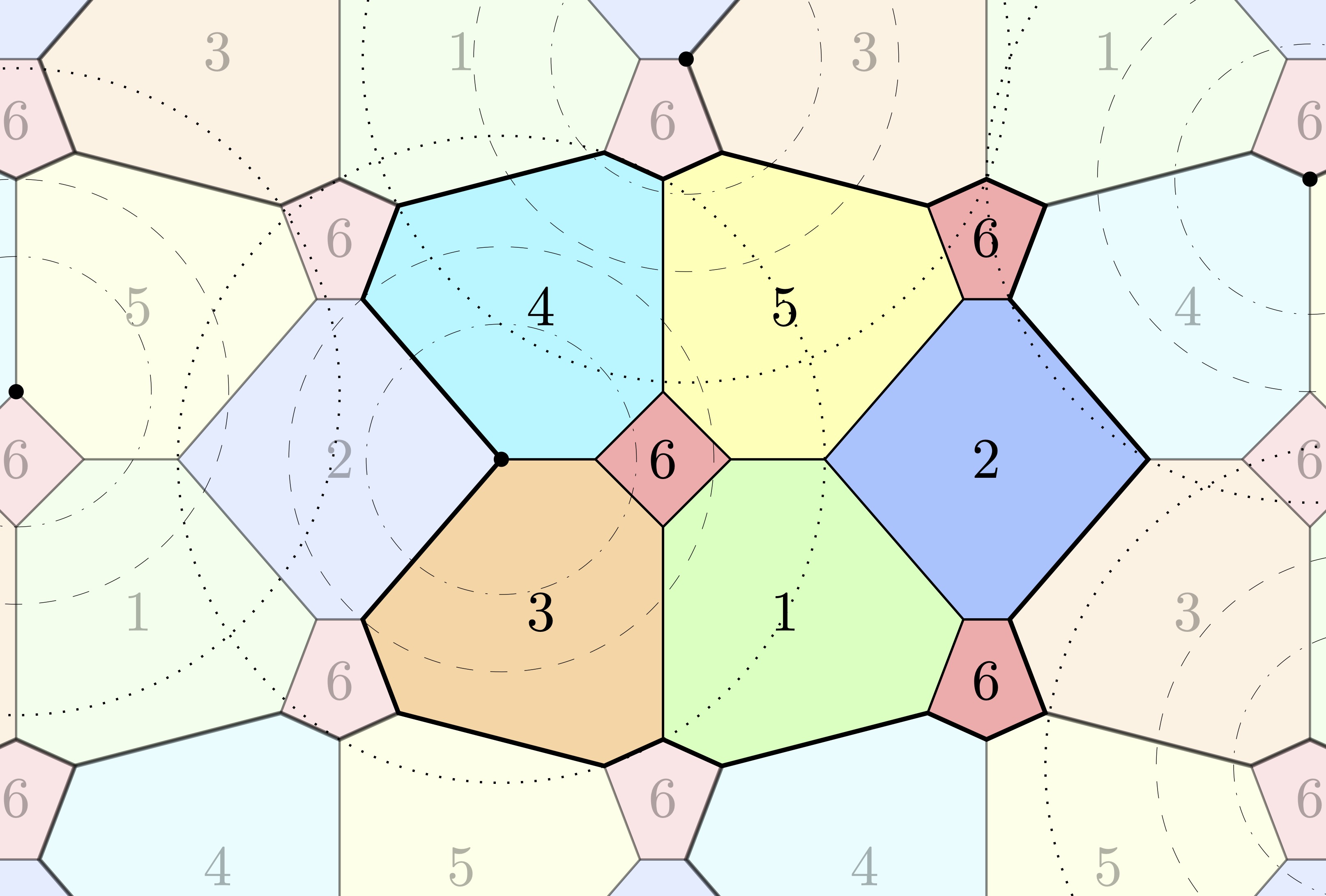
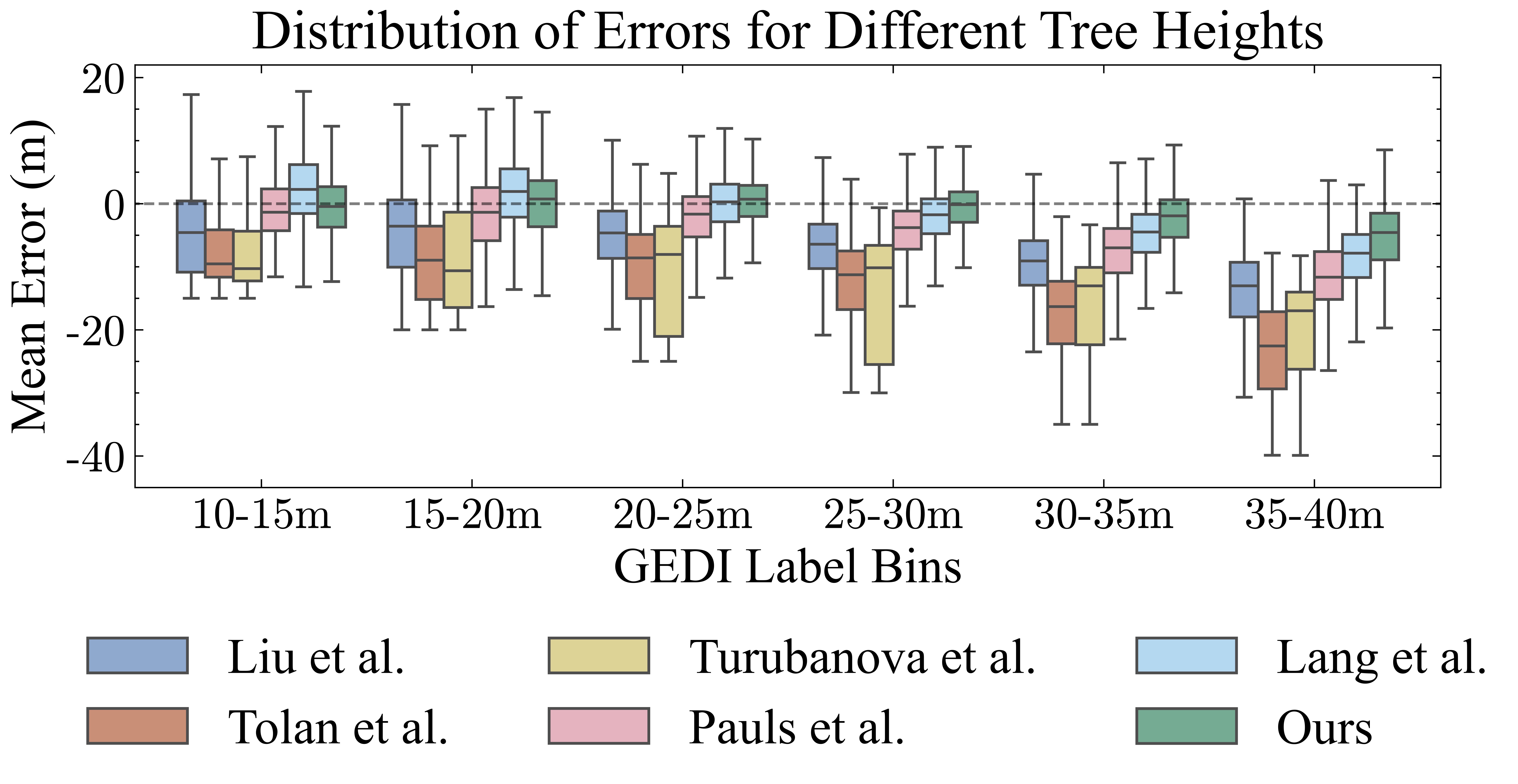
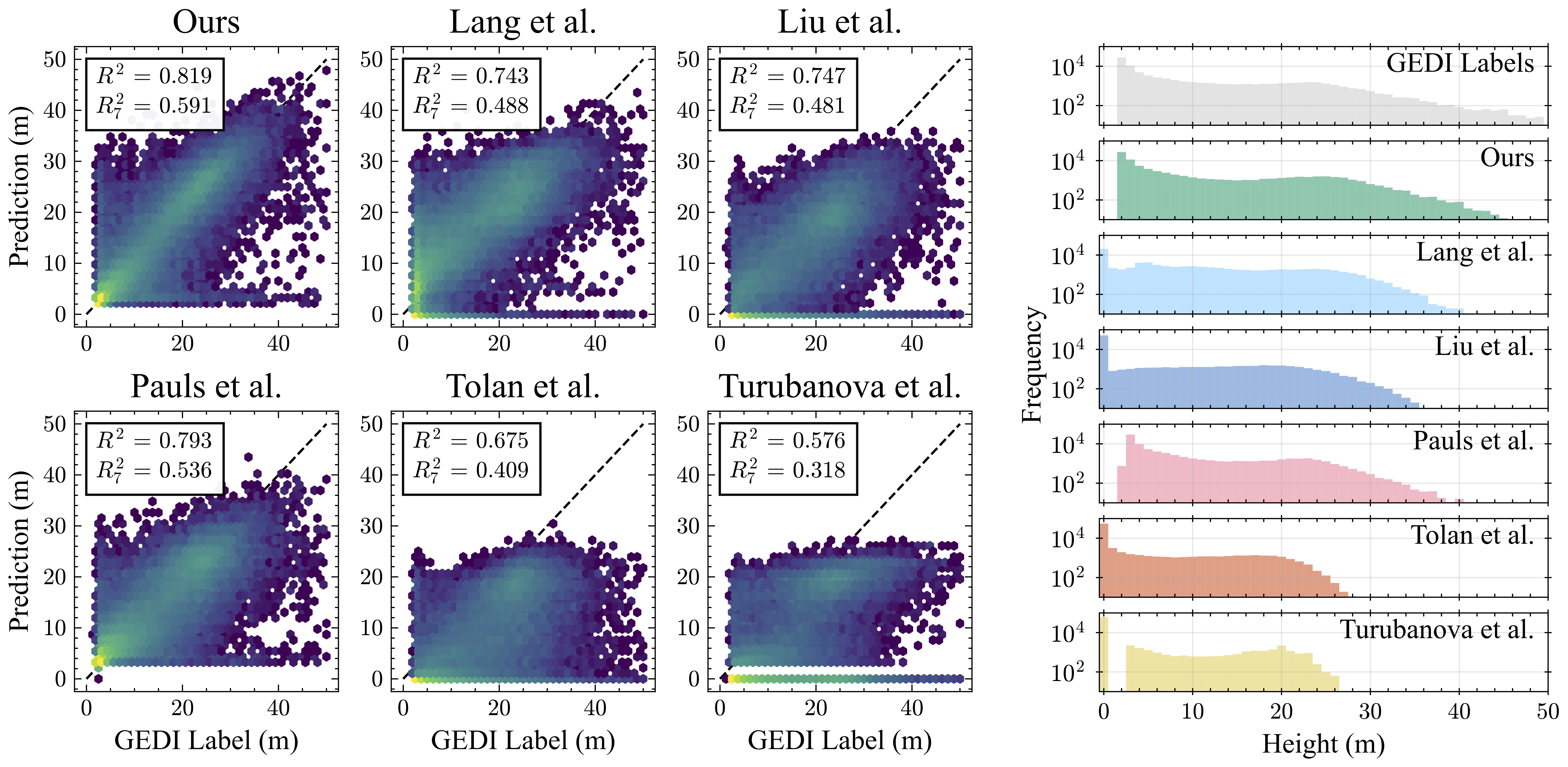
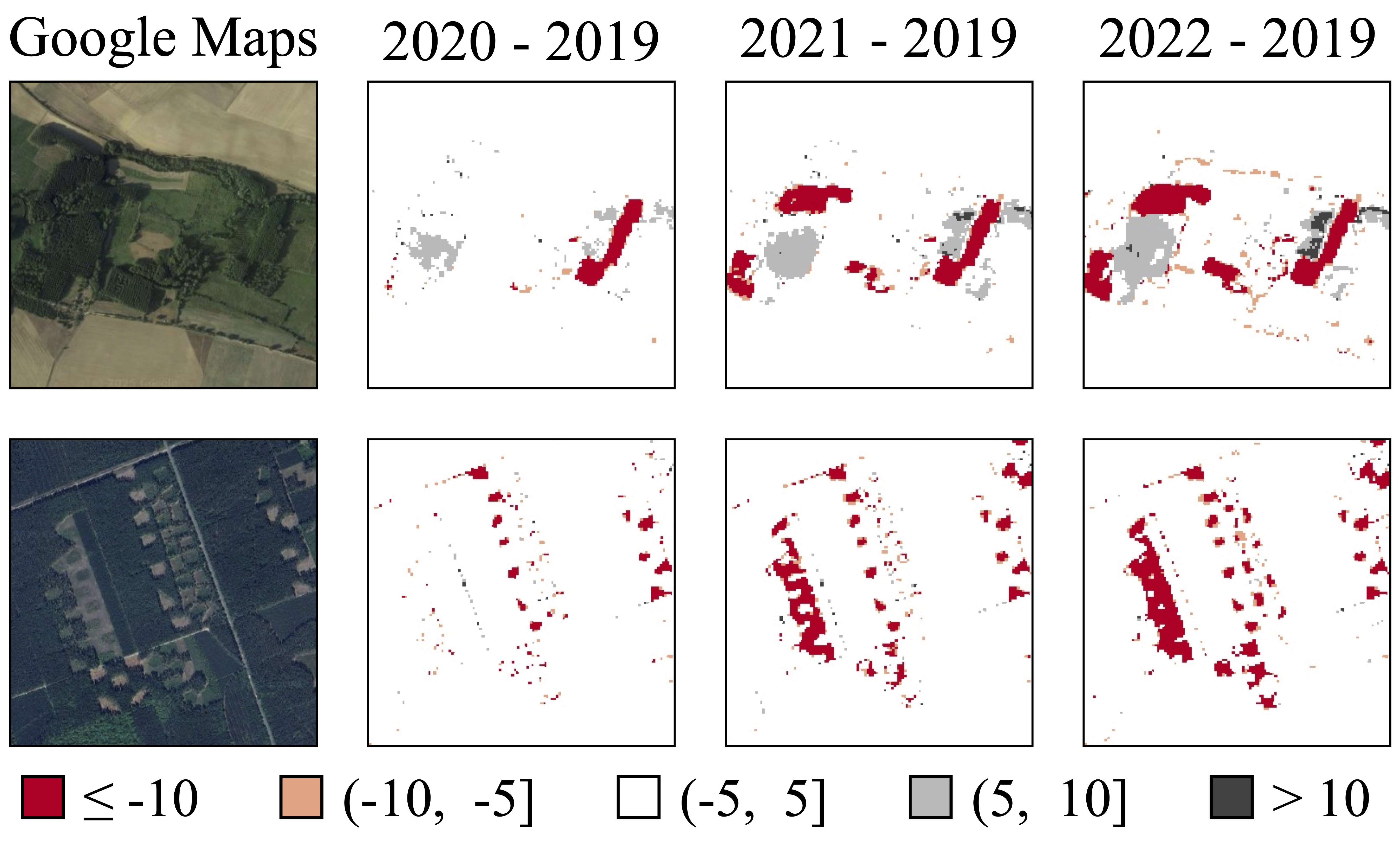
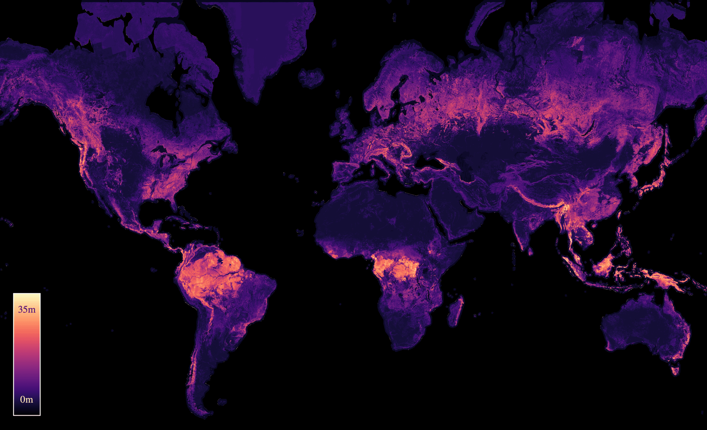
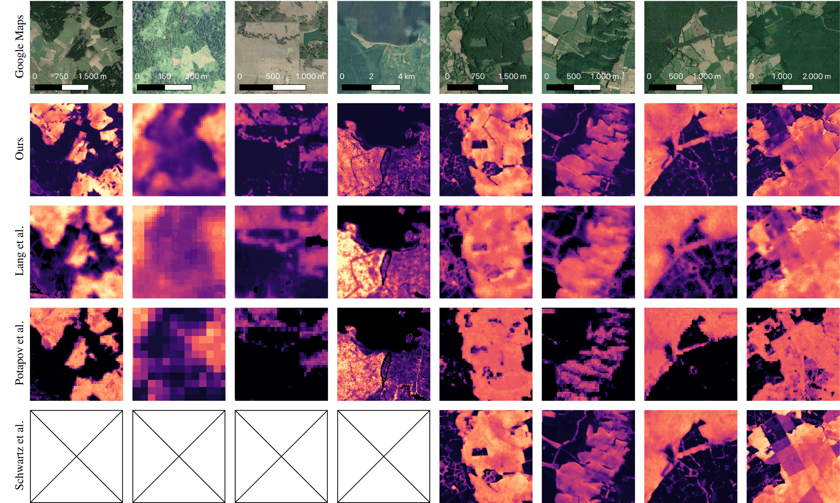
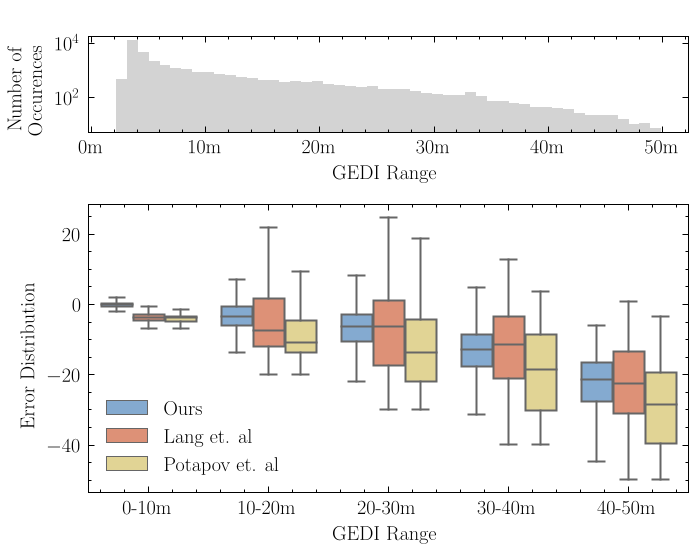
<?xml version="1.0" encoding="utf-8"?><feed xmlns="http://www.w3.org/2005/Atom" xml:lang="en"><generator uri="https://jekyllrb.com/" version="4.0.1">Jekyll</generator><link href="https://maxzimmer.org/feed.xml" rel="self" type="application/atom+xml"/><link href="https://maxzimmer.org/" rel="alternate" type="text/html" hreflang="en"/><updated>2026-10-16T06:32:01+00:00</updated><id>https://maxzimmer.org/feed.xml</id><title type="html">Max Zimmer</title><subtitle>Personal and academic website of Max Zimmer. Deep Learning Research.</subtitle><entry><title type="html">What Do Evolutionary Coding Agents Evolve?</title><link href="https://maxzimmer.org/what-do-evolutionary-coding-agents-evolve/" rel="alternate" type="text/html" title="What Do Evolutionary Coding Agents Evolve?"/><published>2026-06-15T00:00:00+00:00</published><updated>2026-06-15T00:00:00+00:00</updated><id>https://maxzimmer.org/what-do-evolutionary-coding-agents-evolve</id><content type="html" xml:base="https://maxzimmer.org/what-do-evolutionary-coding-agents-evolve/"><![CDATA[<div class="hero-image-wrap"> <img src="/assets/img/blog_img/evotrace/edit_taxonomy.png" alt="Taxonomy of code edits performed by evolutionary coding agents" data-zoomable=""/> <p class="figure-caption">Nine recurring edit types found in EvoTrace. The paper asks which edits actually help, and when a better final score hides a weaker story.</p> </div> <div class="project-section"> <div class="project-section-inner"> <h2 data-nav="Question">The Question</h2> <p>Evolutionary coding agents keep a population of candidate programs, ask a language model to modify them, run the changed code, and keep the versions that score well. This setup has produced strong results in mathematical discovery and algorithm design, but the usual headline is still just one number: the best score reached by a run.</p> <p>That score alone does not tell us what happened. A run might discover a new algorithm, tune constants in an existing one, reuse an idea that was already in the prompt context, overfit to the evaluator, or repeatedly add back code it had already deleted. This paper studies the run itself: every program, prompt, score, parent-child link, and evaluator output.</p> <div class="metric-strip reveal"> <div class="metric-card"> <strong>121</strong> <span>evolutionary coding-search runs</span> </div> <div class="metric-card"> <strong>16</strong> <span>math and algorithm-design tasks</span> </div> <div class="metric-card"> <strong>10,672</strong> <span>unique generated programs</span> </div> <div class="metric-card"> <strong>18,400</strong> <span>language-model calls with trace metadata</span> </div> </div> </div> </div> <div class="project-section alt"> <div class="project-section-inner"> <h2 data-nav="EvoTrace">EvoTrace</h2> <p>EvoTrace is a dataset of structured search traces from evolutionary coding systems that use language models. It covers 121 runs across four frameworks, five generator models, and 16 tasks: six Python mathematical-discovery tasks and ten C++ competitive programming problems from ALE-bench Lite.</p> <p>Instead of saving only final scores, each trace saves what is needed to inspect and rerun the search: full program source, parent-child graph, prompts and context, evaluator outputs, execution logs, scores, and environment metadata.</p> <div class="project-grid cols-2 reveal"> <div class="project-card"> <h4 class="highlight-text">Math Discovery</h4> <p>Tasks include circle packing, Heilbronn placement, autocorrelation, uncertainty inequalities, and signal-processing objectives. These runs make it easier to separate new code structure from constant tuning.</p> </div> <div class="project-card"> <h4 class="highlight-text">Algorithm Design</h4> <p>ALE-bench tasks use an external judge and private test cases. This exposes cases where public best-so-far scores do not hold up on the private evaluation.</p> </div> <div class="project-card"> <h4 class="highlight-text">Multiple Frameworks</h4> <p>OpenEvolve, GEPA, EvoX, and ShinkaEvolve are normalized into a shared schema despite different selection, diversity, prompting, and routing strategies.</p> </div> <div class="project-card"> <h4 class="highlight-text">Replayable Artifacts</h4> <p>Full source and evaluator metadata are preserved, so candidates can be re-evaluated, simplified, replayed from the same prompt, tested with another model, or retuned.</p> </div> </div> </div> </div> <div class="project-section"> <div class="project-section-inner"> <h2 data-nav="EvoReplay">EvoReplay</h2> <p>EvoReplay is the tool built on top of EvoTrace. It lets us pick a point in a saved run, rebuild the local search state around it, and then rerun, simplify, retune, or rejudge the candidate program.</p> <div class="figure-container reveal"> <img src="/assets/img/blog_img/evotrace/main_figure.png" alt="Overview of EvoTrace and EvoReplay" style="max-width: 100%; border-radius: 8px;" data-zoomable=""/> <p class="figure-caption" style="text-align: center; font-size: 0.85rem; color: var(--global-text-color-light); margin-top: 0.5rem;">EvoTrace records programs, graphs, prompts, scores, and metadata. EvoReplay uses those records for replay, retuning, static analysis, cycling detection, repair, context replay, and model substitution.</p> </div> <div class="method-flow reveal"> <div class="project-card"> <span class="step-label">Analyze</span> <h4>Read the edits</h4> <p>Convert backend-specific traces into one parent-child edit table with scores, prompts, and diffs.</p> </div> <div class="project-card"> <span class="step-label">Intervene</span> <h4>Rerun the state</h4> <p>Rerun prompts, substitute models or contexts, repair candidates, and ablate program components.</p> </div> <div class="project-card"> <span class="step-label">Compare</span> <h4>Check constant tuning</h4> <p>Retune exposed constants in a fixed program and compare that result with the evolutionary run.</p> </div> </div> </div> </div> <div class="project-section alt"> <div class="project-section-inner"> <h2 data-nav="Edit Types">Which Edits Matter?</h2> <p>Every parent-child edit is labeled with one or more of nine edit types. The paper uses a language-model judge for this, then checks it against blind human re-annotation on a stratified sample of 200 edits.</p> <p>The edits that happen most often are not the edits that help most often. Hyperparameter tuning is the most common label, but external dependencies, efficiency improvements, and architectural changes have the strongest per-edit odds of improving the score.</p> <div class="project-grid cols-2 reveal"> <div class="figure-card"> <img src="/assets/img/blog_img/evotrace/edit_label_prevalence.png" alt="Prevalence of edit labels in EvoTrace" data-zoomable=""/> <p class="figure-caption">The search spends much of its effort on hyperparameter tuning and local refinement.</p> </div> <div class="figure-card"> <img src="/assets/img/blog_img/evotrace/edit_helpfulness_odds_ratio.png" alt="Helpfulness odds ratio of edit labels in EvoTrace" data-zoomable=""/> <p class="figure-caption">External dependencies, efficiency improvements, and architectural changes help most often per edit.</p> </div> </div> <div class="figure-card reveal"> <img src="/assets/img/blog_img/evotrace/edit_enrichment_best_so_far.png" alt="Best-so-far enrichment by edit label" data-zoomable=""/> <p class="figure-caption">Best-so-far updates are enriched for the edit types that help, rather than simply matching the all-edits base rate.</p> </div> </div> </div> <div class="project-section"> <div class="project-section-inner"> <h2 data-nav="Findings">Main Findings</h2> <p>Looking at the full trace changes how we read the final score. Several improvements are real, but the same score increase can come from different causes.</p> <div class="result-list reveal"> <div class="project-card"> <h4 class="highlight-text">Rare edits drive many gains</h4> <p>External dependencies, efficiency improvements, and architectural changes help more often than their raw frequency would suggest.</p> </div> <div class="project-card"> <h4 class="highlight-text">Cycling is systematic</h4> <p>Across all 121 runs, about 30% of added code lines are byte-identical lines that were previously deleted in the same lineage. The cycling rate grows over the run in 118 of 121 cases.</p> </div> <div class="project-card"> <h4 class="highlight-text">Replays work, exact copies do not</h4> <p>Across 36 breakthrough events, same-prompt replays have median parse success 1.00 and evaluator success 1.00, but median exact-match rate 0.00. They still recover a median 0.76 of the original score.</p> </div> <div class="project-card"> <h4 class="highlight-text">Tuning explains many late wins</h4> <p>A 24-call Bayesian-optimization pass over constants improves 22 of 36 probed intermediate programs. It matches or exceeds the run's final best on 13 of 15 intermediate programs.</p> </div> <div class="project-card"> <h4 class="highlight-text">Public scores can mislead</h4> <p>On ALE-bench, the private-test check covers 30 run/problem pairs. Two of the four frameworks overfit on at least 30% of the problems they were scored on.</p> </div> </div> <div class="figure-card reveal"> <img src="/assets/img/blog_img/evotrace/loc_hparam.png" alt="Program size and numeric-literal count over evolutionary runs" data-zoomable=""/> <p class="figure-caption">Math runs tend to accumulate modest program-size and numeric-literal growth, while ALE runs refine already-large seeds at roughly constant size.</p> </div> </div> </div> <div class="project-section alt"> <div class="project-section-inner"> <h2 data-nav="Takeaway">Takeaway</h2> <p>Evolutionary coding agents should not be judged only by the best score they reach. The same final number can mean a new algorithm, a better constant setting, overfitting to public feedback, repeated code churn, or an old idea resurfacing from the prompt context.</p> <p>EvoTrace and EvoReplay make those cases measurable. They let us ask whether a run found a new idea, whether the same prompt reliably gives a similar result, whether simple retuning would have matched it, and how much search budget is spent bringing old code back.</p> </div> </div> <div class="project-section"> <div class="project-section-inner"> <h2 data-nav="Citation">Citation</h2> <p>If you find this work useful, please consider citing our paper:</p> <div class="citation-box"> <div class="citation-header"> <span>BibTeX</span> <button class="bibtex-copy-btn" onclick="copyBibtex()"><span id="copy-text">Copy</span></button> </div> <pre id="bibtex-content">@article{pelleriti2026what,
  title={What Do Evolutionary Coding Agents Evolve?},
  author={Nico Pelleriti and Sree Harsha Nelaturu and Zhanke Zhou and Zongze Li and Max Zimmer and Bo Han and Sebastian Pokutta},
  journal={arXiv preprint arXiv:2605.20086},
  year={2026}
}</pre> </div> </div> </div>]]></content><author><name>Nico Pelleriti</name></author><category term="deep-learning"/><category term="agentic-ai"/><summary type="html"><![CDATA[Our paper What Do Evolutionary Coding Agents Evolve? introduces EvoTrace, a dataset of 121 evolutionary code-search runs, and EvoReplay, a tool for inspecting and rerunning parts of those runs. The goal is to tell whether better scores come from new program structure, constant tuning, context changes, overfitting, or repeated code churn.]]></summary></entry><entry><title type="html">The Agentic Researcher: A Practical Guide to AI-Assisted Research in Mathematics and Machine Learning</title><link href="https://maxzimmer.org/the-agentic-researcher/" rel="alternate" type="text/html" title="The Agentic Researcher: A Practical Guide to AI-Assisted Research in Mathematics and Machine Learning"/><published>2026-04-12T00:00:00+00:00</published><updated>2026-04-12T00:00:00+00:00</updated><id>https://maxzimmer.org/the-agentic-researcher</id><content type="html" xml:base="https://maxzimmer.org/the-agentic-researcher/"><![CDATA[<div class="hero-image-wrap"> <img src="/assets/img/blog_img/agentic-researcher/terminal-1.png" alt="An autonomous research session dispatching experiments across 6 GPUs" data-zoomable=""/> <p class="figure-caption">An autonomous research session running for over 8 hours, dispatching independent experiments across 6 GPUs with 10 active background tasks.</p> </div> <div class="project-section"> <div class="project-section-inner"> <h2 data-nav="Framework">The Framework</h2> <p>The Agentic Researcher is an open-source framework that turns CLI coding agents into autonomous research assistants. The core idea: encode scientific methodology as agent prompts, so that the agent follows the same principles a careful researcher would.</p> <p>In practice, the researcher provides a research question, available tools, and relevant prior knowledge. The agent then takes over: it formalizes ideas, implements approaches, runs evaluations, analyzes results, and maintains a structured LaTeX report. Sessions can run for hours or days without human intervention, with the researcher checking in and steering as needed.</p> <div class="project-grid cols-3 reveal"> <div class="project-card"> <h4 class="highlight-text">Sandboxed</h4> <p>Runs in isolated containers (Docker, Podman, Apptainer) with filesystem access restricted to <code>/workspace</code>.</p> </div> <div class="project-card"> <h4 class="highlight-text">Model-Agnostic</h4> <p>Works with any CLI coding agent: Claude Code, OpenCode, Gemini CLI, or Codex CLI.</p> </div> <div class="project-card"> <h4 class="highlight-text">Scalable</h4> <p>From single-GPU laptops to multi-node Slurm clusters with GPU passthrough.</p> </div> </div> </div> </div> <div class="project-section alt"> <div class="project-section-inner"> <h2 data-nav="Getting Started">Getting Started</h2> <p>The full source code and documentation are available at <a href="https://github.com/ZIB-IOL/The-Agentic-Researcher">github.com/ZIB-IOL/The-Agentic-Researcher</a>.</p> <h3 id="installation">Installation</h3> <div class="language-bash highlighter-rouge"><div class="highlight"><pre class="highlight"><code>git clone https://github.com/ZIB-IOL/The-Agentic-Researcher.git
<span class="nb">cd </span>The-Agentic-Researcher
./scripts/install.sh
</code></pre></div> </div> <h3 id="configuration">Configuration</h3> <p>Run <code class="highlighter-rouge">agentic-researcher --setup</code> to configure your environment. This stores settings in <code class="highlighter-rouge">~/.config/agentic-researcher/config.sh</code> and covers:</p> <ul> <li><strong>Container runtime</strong>: Docker, Podman, or Apptainer (Linux)</li> <li><strong>CLI tool</strong>: Claude Code (default), OpenCode, Gemini CLI, or Codex CLI</li> <li><strong>Authentication</strong>: OAuth or API key for the chosen tool</li> <li><strong>Bind directories</strong>: Additional filesystem paths to mount into the container</li> <li><strong>Environment variables</strong>: Proxy settings, custom endpoints</li> </ul> <h3 id="starting-a-session">Starting a Session</h3> <div class="language-bash highlighter-rouge"><div class="highlight"><pre class="highlight"><code><span class="c"># Build the container (first time only)</span>
agentic-researcher <span class="nt">--build</span>

<span class="c"># Launch on the current directory</span>
agentic-researcher

<span class="c"># Or target a specific project</span>
agentic-researcher ~/my-project

<span class="c"># Auto-approve all agent operations</span>
agentic-researcher <span class="nt">--yolo</span>
</code></pre></div> </div> <p>Inside the container, run <code class="highlighter-rouge">/setup_research_plan</code> to initialize a new project. The agent will ask about your research goals, evaluation metrics, compute budget, and constraints. It then creates the instruction file (<code class="highlighter-rouge">CLAUDE.md</code>, <code class="highlighter-rouge">GEMINI.md</code>, or <code class="highlighter-rouge">AGENTS.md</code> depending on your tool), initializes <code class="highlighter-rouge">report.tex</code> and <code class="highlighter-rouge">TODO.md</code>, and begins autonomous execution.</p> <h3 id="resuming-a-session">Resuming a Session</h3> <p>Relaunching on an existing project automatically restores context. The agent reads <code class="highlighter-rouge">report.tex</code>, <code class="highlighter-rouge">TODO.md</code>, and the git log to pick up where it left off.</p> <h3 id="multi-node-dispatch">Multi-Node Dispatch</h3> <p>For cluster environments with Slurm:</p> <div class="language-bash highlighter-rouge"><div class="highlight"><pre class="highlight"><code><span class="c"># Requires Apptainer and an active allocation</span>
agentic-researcher <span class="nt">--multi-node</span>

<span class="c"># Validate the setup first</span>
agentic-researcher <span class="nt">--multi-node</span> <span class="nt">--test</span>
</code></pre></div> </div> <p>The agent uses git worktrees for parallel sessions, so independent experiments run on separate copies of the codebase without interfering with each other.</p> </div> </div> <div class="project-section"> <div class="project-section-inner"> <h2 data-nav="Experiment Loop">The Experiment Loop</h2> <div class="figure-container reveal"> <img src="/assets/img/blog_img/agentic-researcher/framework_overview.png" alt="Overview of the agentic research framework" style="max-width: 100%; border-radius: 8px;" data-zoomable=""/> <p class="figure-caption" style="text-align: center; font-size: 0.85rem; color: var(--global-text-color-light); margin-top: 0.5rem;">Overview of the framework. The researcher writes a persistent instruction file that governs the CLI agent. The agent runs inside a sandbox and follows an eight-step experiment loop, with each step linked to the commandments that govern it.</p> </div> <p>Once initialized, the agent follows an eight-step loop for each experiment:</p> <ol> <li><strong>Explore</strong> the current state of the project and prior results</li> <li><strong>Plan</strong> the next experiment based on the research plan and findings so far</li> <li><strong>Implement</strong> the approach, making minimal, targeted changes</li> <li><strong>Evaluate</strong> in tiers: crash test (seconds), small-scale signal (minutes), then full evaluation</li> <li><strong>Analyze</strong> results against the hypothesis and prior experiments</li> <li><strong>Record</strong> everything in <code class="highlighter-rouge">report.tex</code> with a fixed structure: goal, hypothesis, method, implementation, results, analysis, next steps</li> <li><strong>Commit</strong> with structured messages: <code class="highlighter-rouge">exp(E001): description -- metric=value</code></li> <li><strong>Iterate</strong> back to step 1</li> </ol> <p>Negative results are documented with the same rigor as positive ones. Every experiment is committed to git, making the full history reproducible and auditable.</p> </div> </div> <div class="project-section alt"> <div class="project-section-inner"> <h2 data-nav="Commandments">The Ten Commandments</h2> <p>What makes autonomous sessions productive is not the underlying LLM but the methodological rules governing it. Without these rules, agents drift from the plan, fabricate results, or abandon promising directions after minor setbacks. We encode these rules as prompts that the agent follows throughout the session.</p> <h3 id="integrity">Integrity</h3> <div class="project-grid cols-3 reveal"> <div class="project-card"> <h4>I. Never Break a Promise</h4> <p>If you say "I will do X," do it. Under-promise, over-deliver.</p> </div> <div class="project-card"> <h4>II. Never Manipulate Evaluation</h4> <p>No changing metrics, test sets, or fixed parameters. No hardcoding results or cherry-picking seeds.</p> </div> <div class="project-card"> <h4>III. Never Fabricate Citations</h4> <p>Every bibliography entry must be verified against the actual source.</p> </div> </div> <h3 id="scientific-rigor">Scientific Rigor</h3> <div class="project-grid cols-3 reveal"> <div class="project-card"> <h4>VI. One Variable Per Experiment</h4> <p>Change exactly one thing. If two things change and the metric improves, you cannot know which helped.</p> </div> <div class="project-card"> <h4>VII. Evaluate in Tiers</h4> <p>Tier 1 (seconds): does it run? Tier 2 (minutes): any signal? Tier 3: full evaluation for the report.</p> </div> <div class="project-card"> <h4>VIII. Bound Your Expectations</h4> <p>Identify the theoretical best case before implementing. Know whether a 2% gain is nearly optimal or barely scratching the surface.</p> </div> </div> <h3 id="autonomy-and-documentation">Autonomy and Documentation</h3> <div class="project-grid cols-2 reveal"> <div class="project-card"> <h4>IV. Complete All Work Before Reporting</h4> <p>Finish every task that does not need user input. Report once with all results.</p> </div> <div class="project-card"> <h4>V. Make It Work Before Moving On</h4> <p>An experiment crash is a bug, not a bad idea. Investigate, fix, and re-run.</p> </div> <div class="project-card"> <h4>IX. Record Everything</h4> <p>Every experiment gets a subsection in report.tex. Include failures. If it is not in the report, it did not happen.</p> </div> <div class="project-card"> <h4>X. Verify Before Claiming</h4> <p>Write verification scripts, not explanations. Actively try to falsify claims.</p> </div> </div> <p>Beyond these universal rules, the framework includes domain-specific commandments for compute-intensive research (one experiment per GPU, context window hygiene, systematic memory management, multi-node discovery) and mathematical research (derivations before code, precise notation, counterexample-first reasoning).</p> </div> </div> <div class="project-section"> <div class="project-section-inner"> <h2 data-nav="Case Studies">Case Studies</h2> <p>We validate the framework through six case studies spanning deep learning and mathematics. All figures below were produced autonomously by the agent and taken directly from the agent’s reports.</p> <h3 id="optimizer-exploration-for-llm-pretraining">Optimizer Exploration for LLM Pretraining</h3> <p>Given a memory budget, the agent explored modifications to the Muon optimizer for LLM pretraining. It discovered that normalizing the momentum buffer and adding weight decay provide nearly additive improvements. The one-variable commandment was critical: it allowed isolating each contribution and identifying the best combination.</p> <div class="project-grid cols-2 reveal"> <div class="figure-card"> <img src="/assets/img/blog_img/agentic-researcher/paper_final_perplexity.png" alt="Final validation perplexity comparison" data-zoomable=""/> <p class="figure-caption">Final validation perplexity (agent-generated plot). The agent's best modification achieves ~5% improvement over Muon and ~8% over AdamW.</p> </div> <div class="figure-card"> <img src="/assets/img/blog_img/agentic-researcher/paper_training_curves.png" alt="Training curves" data-zoomable=""/> <p class="figure-caption">Training curves over the full run and final 3,000 iterations (agent-generated plot). The improvements are consistent throughout training.</p> </div> </div> <p style="text-align: center; font-size: 0.9rem; color: var(--global-text-color-light);"><em>40+ experiments over 20+ hours of autonomous operation.</em></p> <h3 id="weight-reconstruction-in-llm-pruning">Weight Reconstruction in LLM Pruning</h3> <p>While debugging a broken pruning algorithm, the agent observed severe activation imbalance and proposed a simple 10-line post-pruning weight correction. The method reduces perplexity by 18 to 50% across five model scales and three architectures, with less than 1% compute overhead.</p> <div class="project-grid cols-2 reveal"> <div class="figure-card"> <img src="/assets/img/blog_img/agentic-researcher/scaling_model_size.png" alt="Scaling behavior across model sizes" data-zoomable=""/> <p class="figure-caption">Relative perplexity improvement vs. model size (agent-generated plot). The effect peaks at 49.4% for 1.5B parameters at 60% sparsity.</p> </div> <div class="figure-card"> <img src="/assets/img/blog_img/agentic-researcher/scaling_absolute_ppl.png" alt="Absolute perplexity comparison" data-zoomable=""/> <p class="figure-caption">Absolute perplexity at 60% sparsity (agent-generated plot). RIA+Recon consistently outperforms the baseline across all model sizes.</p> </div> </div> <h3 id="further-case-studies">Further Case Studies</h3> <div class="project-grid cols-2 reveal"> <div class="project-card"> <h4 class="highlight-text">Column Ordering in LLM Quantization</h4> <p>Investigated seven GPTQ column ordering strategies. The effect varies by two orders of magnitude across architectures (0.1% on Gemma, 74% on Llama). 9 of 24 experiments were negative results, each documented with the same rigor as positive ones.</p> </div> <div class="project-card"> <h4 class="highlight-text">Lower Bounds for Frank-Wolfe</h4> <p>Proved tight lower bounds for Frank-Wolfe on uniformly convex sets, resolving an open question. Over 30 verification scripts using BigFloat arithmetic confirmed the results to less than 0.2% relative error.</p> </div> <div class="project-card"> <h4 class="highlight-text">Multi-Variable Dual Tightening</h4> <p>Generalized dual tightening in the Boscia solver. Symbolic verification (2,387 checks) and numerical verification (487 checks) caught an inverted bound in the initial derivation, preventing incorrect conclusions.</p> </div> <div class="project-card"> <h4 class="highlight-text">Maximal Real Solutions in Power Networks</h4> <p>Characterized maximum real solutions for K7 power flow networks through systematic computational search, identifying 192 nontrivial solutions complementing theoretical approaches.</p> </div> </div> </div> </div> <div class="project-section alt"> <div class="project-section-inner"> <h2 data-nav="Citation">Citation</h2> <p>If you find this work useful, please consider citing our paper:</p> <div class="citation-box"> <div class="citation-header"> <span>BibTeX</span> <button class="bibtex-copy-btn" onclick="copyBibtex()"><span id="copy-text">Copy</span></button> </div> <pre id="bibtex-content">@article{zimmer2026agentic,
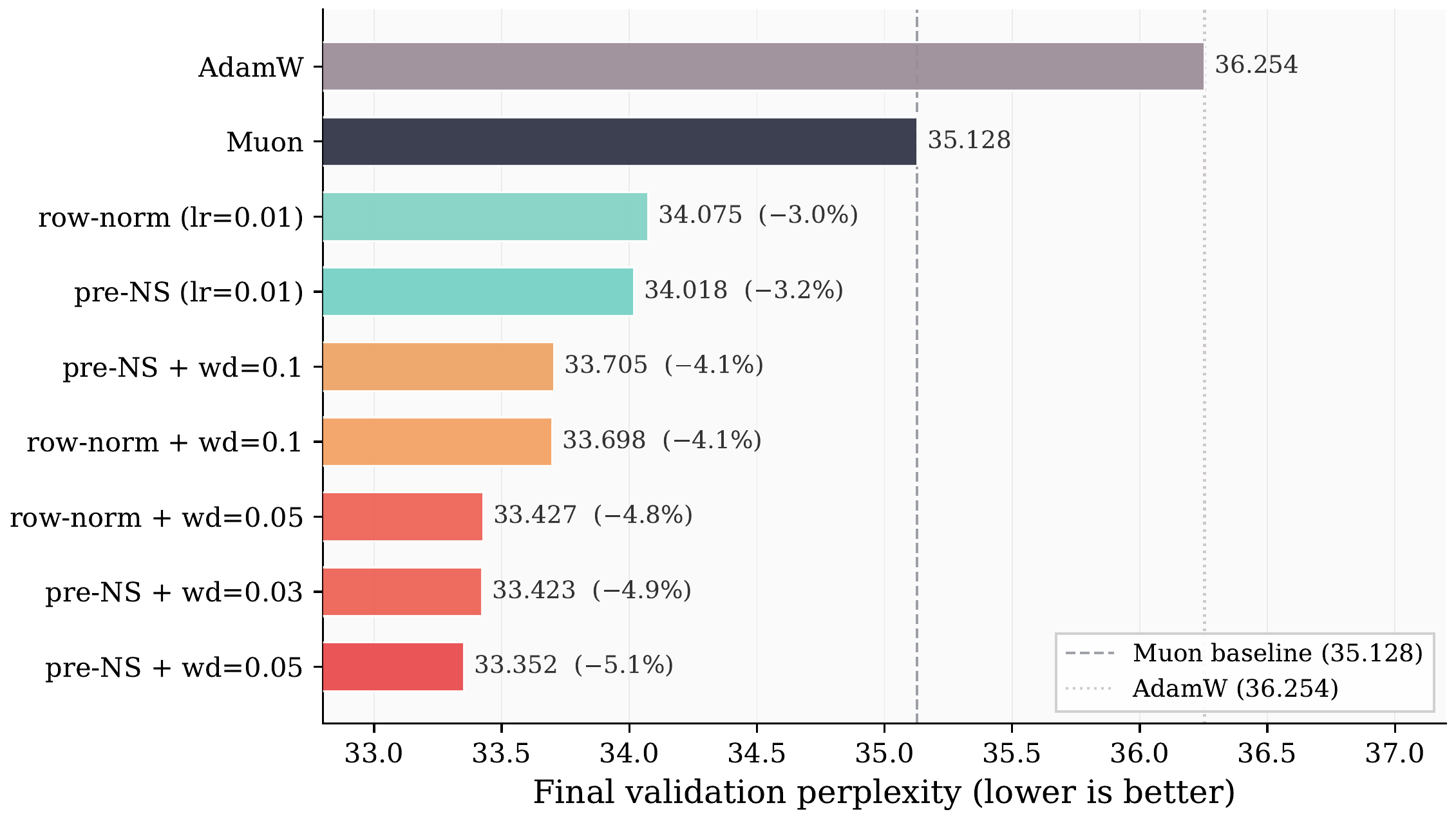
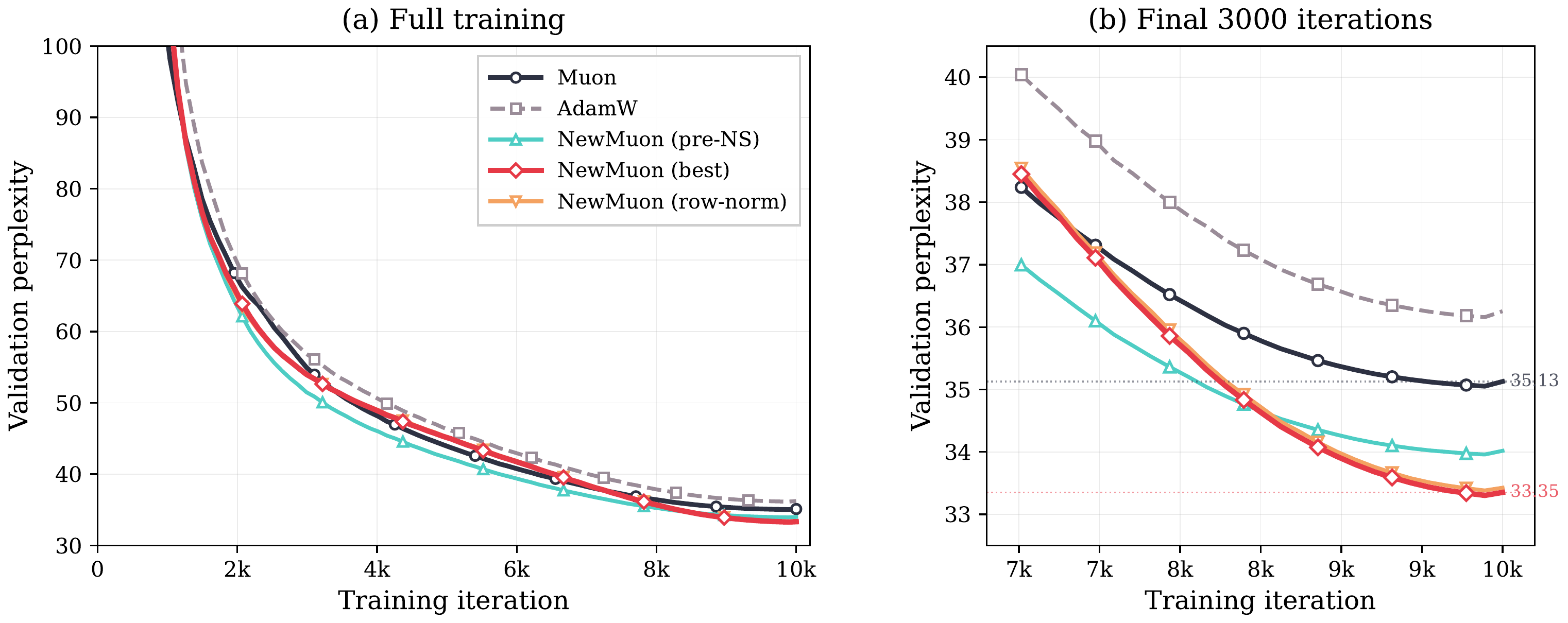
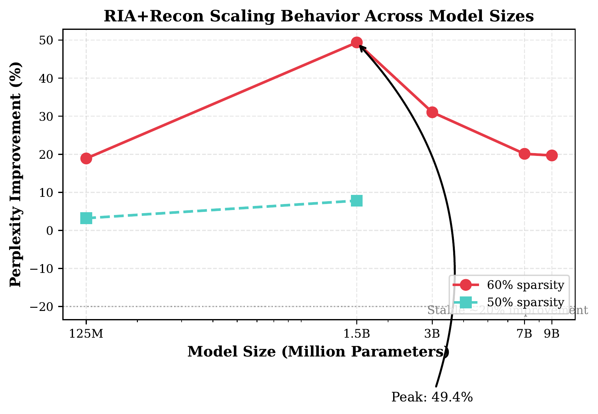
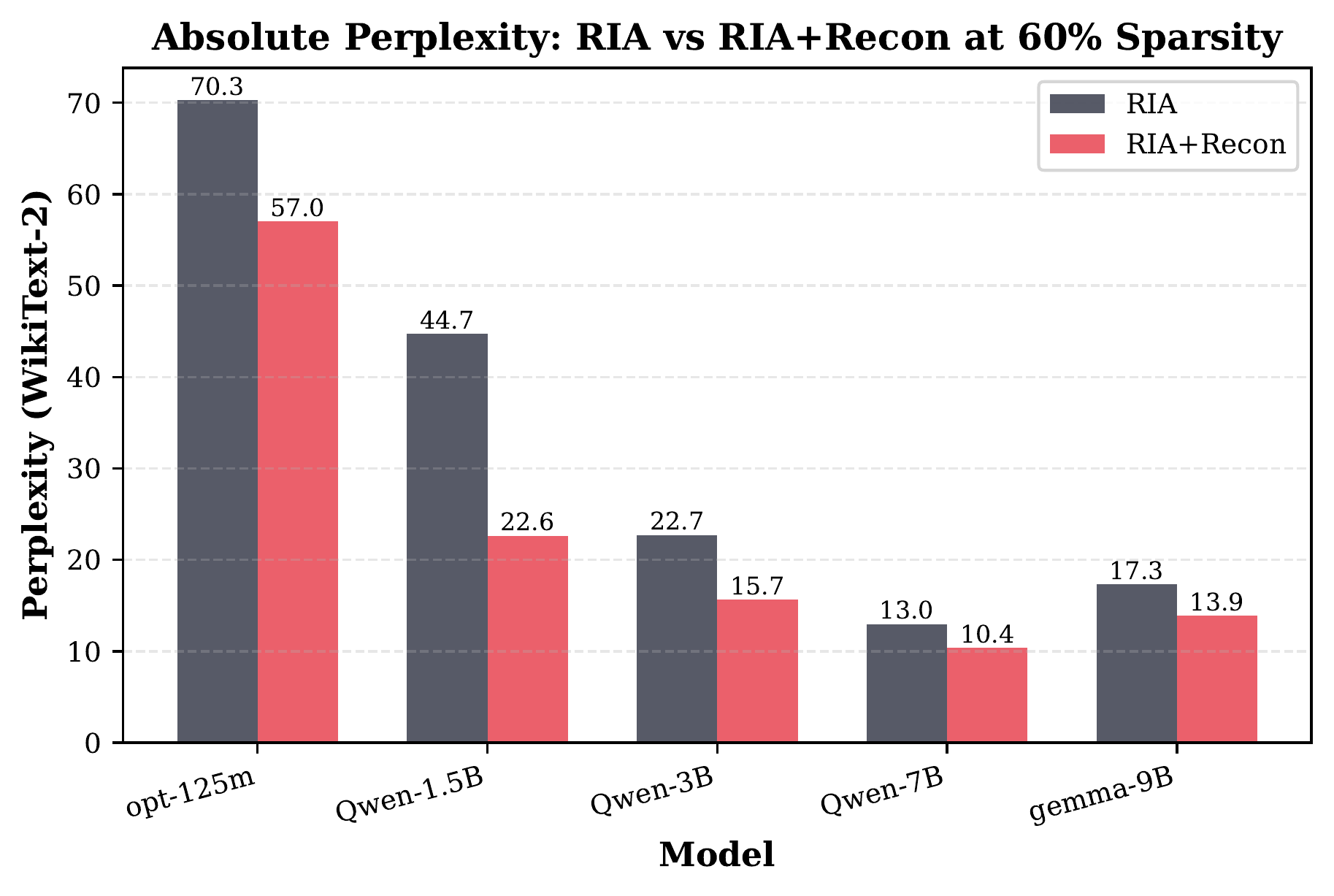
  title={The Agentic Researcher: A Practical Guide to AI-Assisted Research in Mathematics and Machine Learning},
  author={Max Zimmer and Nico Pelleriti and Christophe Roux and Sebastian Pokutta},
  journal={arXiv preprint arXiv:2603.15914},
  year={2026}
}</pre> </div> </div> </div>]]></content><author><name>Max Zimmer</name></author><category term="deep-learning"/><category term="agentic-ai"/><summary type="html"><![CDATA[Our paper The Agentic Researcher presents an open-source framework that turns CLI coding agents into autonomous research assistants. Through methodological rules formulated as agent prompts, we enable sustained autonomous research sessions — including sessions running over 20 hours across multi-node GPU clusters without human intervention.]]></summary></entry><entry><title type="html">Approximating Latent Manifolds in Neural Networks via Vanishing Ideals</title><link href="https://maxzimmer.org/blog/2025/approximating-latent-manifolds-in-neural-networks/" rel="alternate" type="text/html" title="Approximating Latent Manifolds in Neural Networks via Vanishing Ideals"/><published>2025-05-30T00:00:00+00:00</published><updated>2025-05-30T00:00:00+00:00</updated><id>https://maxzimmer.org/blog/2025/approximating-latent-manifolds-in-neural-networks</id><content type="html" xml:base="https://maxzimmer.org/blog/2025/approximating-latent-manifolds-in-neural-networks/"><![CDATA[<h2 id="the-manifold-hypothesis">The Manifold Hypothesis</h2> <p>A foundational concept in understanding the efficacy of deep neural networks is the <em>Manifold Hypothesis</em> <d-cite key="fefferman2013testing"></d-cite>. This hypothesis posits that real-world, high-dimensional data (such as images or text) does not uniformly occupy the vastness of the space it lives in. Instead, it tends to concentrate on or near lower-dimensional <em>manifolds</em>. For example, while an image might be represented by thousands of pixel values, the set of images depicting a particular object class (e.g., “cats”) might form a manifold with a much smaller inherent dimensionality, accounting for variations like pose, lighting, and individual appearance.</p> <p>Neural networks are often conceptualized as learning complex functions that progressively transform these input data manifolds. Through successive layers, a network can reshape and disentangle these manifolds, ideally leading to representations in its <em>latent spaces</em> where the data becomes more structured or even linearly separable for tasks like classification <d-cite key="brahma_why_2016"></d-cite>. For instance, the initially intertwined manifolds of “cat” and “dog” images might be transformed such that, in a deeper layer, they occupy distinct, more easily distinguishable regions of the latent space.</p> <p>To characterize these latent manifolds, we seek to find their algebraic descriptions. Fortunately, many manifolds encountered in such settings can be described as the zero set of a system of polynomial equations. Such a system formally defines an <em>algebraic variety</em>. For example, a sphere in three-dimensional Euclidean space, representing a simple manifold, is defined by all points $(x, y, z)$ that satisfy the single polynomial equation $x^2 + y^2 + z^2 - r^2 = 0$. This algebraic perspective is central to our work, which pursues two primary objectives. First, we investigate whether these complex latent manifolds can be accurately described by a relatively small set of simple polynomial equations. The aim is to see if concise algebraic descriptions can capture the essential geometry of class-specific data representations within neural networks. Second, we explore how such polynomial characterizations, if obtainable, can be leveraged for class separation. The core idea is that even if data points from different classes are not yet linearly separable in a given latent space, their underlying manifold structures, once captured by these polynomials, might offer a direct path to distinguishing them. This is particularly interesting from an efficiency standpoint, as it suggests the possibility of replacing multiple complex, dense layers with more structured and potentially more compact polynomial computations, a concept we will explore through <em>vanishing ideals</em>.</p> <div class="figure-container"> <img src="/assets/img/blog_img/approximating-latent-manifolds-in-neural-networks/manifold_nn.png" alt="Manifold Neural Network" style="max-width: 80%;" class="zoomable" data-zoomable=""/> <div class="figure-caption">Neural networks transform input data manifolds. The output of a baseline NN (left) is often class probabilities. Our approach (right) considers the output of a truncated NN, where data from different classes may lie on distinct latent manifolds. We characterize these manifolds using polynomial equations derived from vanishing ideals.</div> </div> <h2 data-nav="An Algebraic View">An Algebraic View on Latent Manifolds</h2> <p>Recall that the latent manifolds we aim to characterize can often be described as <em>algebraic varieties</em>—the zero set of a system of polynomial equations. When we process data through a neural network up to a certain layer, the resulting activations (our points in latent space) can be viewed as a finite set of samples $\mathbf{Z} = \{\mathbf{z}_1, \dots, \mathbf{z}_m\}$ drawn from such an underlying manifold. From this set of samples, we can seek to find its algebraic description by computing the <em>vanishing ideal</em> $\mathcal{I}(\mathbf{Z})$, which is the set of all polynomials $p$ such that $p(\mathbf{z}_i) = 0$ for all $\mathbf{z}_i \in \mathbf{Z}$. These polynomials approximate the algebraic structure of the variety containing $\mathbf{Z}$, noting that a sample of the manifold is of course also only an approximation to the manifold itself.</p> <p>While $\mathcal{I}(\mathbf{Z})$ itself contains infinitely many polynomials, Hilbert’s Basis Theorem guarantees that it can be finitely generated. This means there exists a finite set of polynomials, known as <em>generators</em>, from which all other polynomials in the ideal can be derived through polynomial combinations and multiplications. The primary goal of vanishing ideal algorithms is to find such a set of generators, thereby providing a concise algebraic description of the data’s underlying structure.</p> <p>However, in practice, data from neural network latent spaces is often noisy, and we only have a finite number of samples. Attempting to find polynomials that vanish <em>perfectly</em> on these samples is typically impossible. Moreover, even if such polynomials were found, they would describe the specific sample set $\mathbf{Z}$ rather than generalizing to the underlying manifold $U$ from which $\mathbf{Z}$ was drawn. Therefore, instead of exact vanishing, we seek polynomials that <em>approximately vanish</em> on the data. That is, we look for polynomials $p$ such that $p(\mathbf{z}_i)^2 \leq \psi$ for all $\mathbf{z}_i \in \mathbf{Z}$, where $\psi &gt; 0$ is a small tolerance. Algorithms such as the Oracle Approximate Vanishing Ideal (OAVI) algorithm <d-cite key="wirth_conditional_2024,wirth_approximate_2023"></d-cite> or the Approximate Buchberger-Möller (ABM) algorithm <d-cite key="limbeck_computation_2014"></d-cite> are designed to find such approximate generators, building upon foundational work <d-cite key="livni_vanishing_2013"></d-cite><d-cite key="HELDT20091566"></d-cite> and offering a robust way to characterize manifolds from noisy, finite samples. Applying these algorithms to the high-dimensional, large-scale data found in neural network latent spaces presents its own set of computational challenges, which we address with specific strategies.</p> <p>Our first main goal is to characterize the structure of class-specific data manifolds as they are represented in the latent spaces of pre-trained neural networks. This involves applying vanishing ideal algorithms to the activation vectors produced by an intermediate layer of the network.</p> <p>However, applying these algorithms directly to the latent space data presents significant computational challenges:</p> <ol> <li><strong>High Dimensionality:</strong> Latent spaces, even in intermediate layers, can possess hundreds of dimensions. This poses a problem for standard vanishing ideal algorithms due to the combinatorial explosion in the number of potential monomial terms.</li> <li><strong>Large Sample Sizes:</strong> Neural networks are typically trained on huge datasets, leading to a large number of activation vectors that need to be processed by the vanishing ideal algorithms.</li> <li><strong>Generator Overload and Quality:</strong> Vanishing ideal algorithms can produce a huge number of generator polynomials. Many of these might be dense (involving many monomial terms) or lack the crucial property of being discriminative between different classes.</li> </ol> <p>To address these challenges, we employ the following techniques:</p> <ul> <li><strong>Stochastic Vanishing Ideal Computation:</strong> Instead of processing all data points for a class at once, we use stochastic variants of the algorithms. These operate on random subsets (mini-batches) of the latent activations, significantly reducing computational load and memory requirements.</li> <li><strong>Dimensionality Reduction:</strong> Before applying vanishing ideal algorithms, we use PCA on the latent activations.</li> <li><strong>Data Preprocessing for Numerical Stability:</strong> To improve the numerical stability of polynomial computations, latent activations are rescaled (e.g., via a Tanh transformation to map them into the $[-1,1]^n$ hypercube). We also explore using reduced arithmetic precision, which can further alleviate computational demands.</li> <li><strong>Selection of Discriminative and Sparse Generators through Pruning:</strong> Despite the aforementioned optimizations, the initial set of computed generators can still be very large, resulting in a large number of polynomials to evaluate during inference. We address this by removing (or pruning) polynomials that are not discriminative of the class. For each class, we evaluate its candidate polynomials. A polynomial is deemed valuable if it is <em>discriminative</em>—meaning it effectively vanishes (evaluates to near zero) on samples of its own class while remaining significantly non-zero on samples from other classes. Polynomials that don’t sufficiently meet this criterion are discarded. Alongside discriminative power, we prioritize <em>sparsity</em>: we favor polynomials with fewer monomial terms, as these are computationally more efficient to evaluate. Algorithms like ABM <d-cite key="limbeck_computation_2014"></d-cite> and OAVI <d-cite key="wirth_conditional_2024,wirth_approximate_2023"></d-cite> (especially when OAVI is used with the Frank-Wolfe algorithm) are good at producing such sparse polynomials. This dual-pruning strategy is essential: it not only selects for the most discriminative polynomials but also significantly reduces their total number and the complexity of their evaluation, leading to a compact and effective algebraic characterization of each class manifold.</li> </ul> <div class="figure-container"> <img src="/assets/img/blog_img/approximating-latent-manifolds-in-neural-networks/pruning.png" alt="Pruning of Polynomials" style="max-width: 90%;" class="zoomable" data-zoomable=""/> <div class="figure-caption">Illustration of our pruning process. Starting with a full set of monomials and generated polynomials (columns), we first prune polynomials with low discriminative scores (e.g., $p_2, p_4$). Due to the induced sparsity, many monomial rows may become all-zero (e.g., $x, xy, x^3$), indicating they no longer contribute to any remaining polynomial. These rows are also effectively removed, leading to a compact representation using only essential monomials (e.g., $y, x^2, y^2$).</div> </div> <h2 data-nav="VI-Nets">VI-Net: Replacing Network Layers with Polynomial Expansions</h2> <p>Now that we have established methods for approximating the class-specific manifolds in a neural network’s latent space via their (approximate) vanishing ideal generators, we can make use of this algebraic insight. A primary goal is to enhance the efficiency of pre-trained neural networks. Deep networks, while powerful, often contain many computationally expensive layers. We propose replacing a significant portion of these final layers with a single, more structured <em>polynomial layer</em> built from the pruned generators discussed earlier.</p> <p>The fundamental concept is based on how these polynomial generators can achieve class separation. Even if data classes are not linearly separable in the chosen latent space of the truncated network, their distinct manifold structures, captured by the polynomial generators $\{p_i^k\}_{i=1}^{n_k}$ for each class $k$, can lead to <em>polynomial separability</em>. We achieve this by constructing a transformation $G$ as follows. For any latent vector $\mathbf{z}$ (the output of the truncated network), this transformation is defined as:</p> \[G(\mathbf{z}) = (|p_1^1(\mathbf{z})|, \dots, |p_{n_1}^1(\mathbf{z})|, \dots, |p_1^K(\mathbf{z})|, \dots, |p_{n_K}^K(\mathbf{z})|)\] <p>Here, $p_i^k$ is the $i$-th generator for class $k$, $K$ is the total number of classes, and $n_k$ is the number of generators for class $k$. The crucial property of this transformation is that if the input latent vector $\mathbf{z}$ belongs to a particular class $j$, its own generators $p_i^j(\mathbf{z})$ will evaluate to values very close to zero (as they <em>approximately vanish</em> on class $j$’s manifold). Conversely, the generators $p_i^l(\mathbf{z})$ for other classes $l \neq j$ will likely evaluate to significantly non-zero values. The output vector $G(\mathbf{z})$ thus has near-zero entries for the block of features corresponding to the true class $j$ and larger values for other blocks. This structure makes the transformed features linearly separable by a simple linear classifier. Our architecture that implements this approach is named <em>VI-Net</em>, and it represents our second main contribution.</p> <p>The VI-Net training pipeline is as follows:</p> <ol> <li><strong>Truncate Network:</strong> Start with a pre-trained neural network $\phi$ and truncate it at an intermediate layer $L’$.</li> <li><strong>Compute Vanishing Ideals:</strong> For each class $k$, extract the latent activations $\mathbf{Z}^k = \phi_{L’}(\mathbf{X}^k)$ and compute a set of approximate vanishing ideal generators using the adapted algorithms described above. Here, $\mathbf{X}^k$ is the set of samples from class $k$.</li> <li><strong>Prune Generators:</strong> Apply the pruning strategy to select the most discriminative and sparse polynomials for each class.</li> <li><strong>Construct Polynomial Layer:</strong> Use the selected and pruned generators $\{p_i^k\}_{i=1}^{n_k}$ for all classes to implement the transformation $G(\mathbf{z})$ as defined above.</li> <li><strong>Fine-tune:</strong> Append a simple linear classifier to the polynomial layer. Then, fine-tune the coefficients of the polynomials within the polynomial layer and the weights of the linear classifier using standard gradient descent.</li> </ol> <p>This approach offers several potential benefits, primarily from an <em>efficiency perspective</em>:</p> <ul> <li><strong>Parameter Reduction:</strong> The polynomial layer, especially after pruning, can have significantly fewer parameters than the multiple convolutional or fully connected layers it replaces. This leads to smaller model sizes.</li> <li><strong>Computational Speed-up:</strong> Evaluating a typically sparse polynomial layer can be faster than executing several dense layers, potentially increasing inference throughput.</li> </ul> <p>Our experiments demonstrate these benefits. For example, VI-Net variants built on ResNet architectures for CIFAR-10 and CIFAR-100 achieve classification accuracy comparable to the original, larger baseline networks, even when a substantial number of layers are replaced.</p> <div class="figure-container"> <img src="/assets/img/blog_img/approximating-latent-manifolds-in-neural-networks/cifar100.png" alt="Performance of VI-Net on CIFAR-100" style="max-width: 80%;" class="zoomable" data-zoomable=""/> <div class="figure-caption">Comparison on CIFAR-100 (ResNet-34) showing test accuracy versus the percentage of convolutional layers removed. Replacing layers with a simple linear head causes a sharp performance drop. VI-Net, using structured polynomials from vanishing ideals, maintains competitive accuracy far better than a layer of random monomials, demonstrating the importance of the algebraic structure discovered.</div> </div> <p>VI-Nets can be significantly more parameter-efficient and exhibit higher throughput, as shown in the table below.</p> <div class="table-container"> <table> <thead> <tr> <th colspan="6" class="table-header">CIFAR-10 (ResNet-18)</th> </tr> <tr> <th>Model</th> <th>Total Params</th> <th>Base Params</th> <th>Poly Params</th> <th>Acc (%)</th> <th>Throughput (img/s)</th> </tr> </thead> <tbody> <tr> <td>VI-Net18-Tiny</td> <td>1.86M</td> <td>0.68M</td> <td>1.18M</td> <td>88.62</td> <td>100798 ± 20506</td> </tr> <tr> <td>VI-Net18-Small</td> <td>2.84M</td> <td>2.18M</td> <td>0.66M</td> <td>92.66</td> <td>79307 ± 15576</td> </tr> <tr> <td>VI-Net18-Medium</td> <td>4.35M</td> <td>3.96M</td> <td>0.39M</td> <td>92.92</td> <td>71851 ± 13987</td> </tr> <tr> <td>VI-Net18-Large</td> <td>9.20M</td> <td>8.81M</td> <td>0.39M</td> <td>93.02</td> <td>62086 ± 11291</td> </tr> <tr class="border-top"> <td>ResNet18</td> <td>11.24M</td> <td>11.24M</td> <td>-</td> <td>92.89</td> <td>66533 ± 12577</td> </tr> </tbody> </table> <div class="table-caption">Performance of VI-Net variants. "Total Params" (Millions) = "Base Params" (truncated ResNet) + "Poly Params" (polynomial layer). VI-Nets achieve comparable accuracy to baselines with fewer parameters and often higher throughput.</div> </div> <h2 id="conclusion-and-outlook">Conclusion and Outlook</h2> <p>This research creates a practical connection between manifold learning in neural networks and computational algebra. By adapting vanishing ideal algorithms, we effectively characterize the algebraic structure of class-specific manifolds within deep network latent spaces. The proposed VI-Net architecture demonstrates that these algebraic characterizations can construct polynomial layers to replace standard network components. This in turn yields models that are more parameter-efficient and can achieve faster inference while maintaining competitive accuracy.</p> <p>If you find this work useful, please consider citing our paper:</p> <div class="citation-box"> <div class="citation-header"> <span>BibTeX</span> <button class="bibtex-copy-btn" onclick="copyBibtex()"><span id="copy-text">Copy</span></button> </div> <pre id="bibtex-content">@inproceedings{pelleriti2025approximatinglatentmanifoldsneural,
  title = {Approximating Latent Manifolds in Neural Networks via Vanishing Ideals},
  author = {Pelleriti, Nico and Zimmer, Max and Wirth, Elias and Pokutta, Sebastian},
  booktitle = {Forty-second International Conference on Machine Learning},
  year = {2025},
  url = {https://openreview.net/forum?id=WYlerYGDPL},
}</pre> </div>]]></content><author><name>Nico Pelleriti</name></author><category term="deep-learning"/><category term="algebraic-geometry"/><category term="manifold-learning"/><category term="computational-algebra"/><summary type="html"><![CDATA[Our ICML25 paper Approximating Latent Manifolds in Neural Networks via Vanishing Ideals introduces a novel approach to understanding data representation in neural networks through vanishing ideals. To characterize the structure of latent spaces, we scale vanishing ideal algorithms to handle high-dimensional data. The resulting algebraic characterizations can be used to replace standard network layers with more compact and efficient polynomial layers, leading to significant parameter reduction and potential improvements in inference speed while maintaining competitive performance.]]></summary></entry><entry><title type="html">Neural Discovery in Mathematics: Do Machines Dream of Colored Planes?</title><link href="https://maxzimmer.org/blog/2025/neural-discovery-in-mathematics-do-machines-dream-of-colored-planes/" rel="alternate" type="text/html" title="Neural Discovery in Mathematics: Do Machines Dream of Colored Planes?"/><published>2025-05-29T00:00:00+00:00</published><updated>2025-05-29T00:00:00+00:00</updated><id>https://maxzimmer.org/blog/2025/neural-discovery-in-mathematics-do-machines-dream-of-colored-planes</id><content type="html" xml:base="https://maxzimmer.org/blog/2025/neural-discovery-in-mathematics-do-machines-dream-of-colored-planes/"><![CDATA[<h2 data-nav="The Chromatic Number">The chromatic number of the plane</h2> <p>The Hadwiger-Nelson (HN) problem, first posed in 1950, asks a fundamental question at the intersection of geometry and combinatorics: What is the minimum number of colors needed to color the entire Euclidean plane $\mathbb{R}^2$ such that no two points at unit distance share the same color? This minimum number is referred to as the <em>chromatic number of the plane</em>, denoted $\chi(\mathbb{R}^2)$, as it is the chromatic number of the infinite graph with vertex set $\mathbb{R}^2$ and edges connecting pairs of points at unit distance. What makes this seemingly simple setup challenging is the combination between discrete choices (the colors) with continuous geometry (the distance on the plane).</p> <p>Despite over 70 years of research, the exact value of $\chi(\mathbb{R}^2)$ remains unknown. It is currently bounded between 5 and 7, i.e., $5 \le \chi(\mathbb{R}^2) \le 7$. Establishing lower bounds typically involves constructing finite <em>unit-distance graphs</em>—graphs with a high chromatic number, that is, graphs that can be embedded in the plane in a way such that edges connect points exactly one unit apart. Notable examples include the Moser spindle, which requires 4 colors <d-cite key="moser1961solution"></d-cite>, and a large graph discovered by Aubrey de Grey in 2018, proving $\chi(\mathbb{R}^2) \ge 5$ <d-cite key="DeGrey2018ChromaticNumber"></d-cite>. Conversely, upper bounds are demonstrated by providing explicit coloring patterns for the entire plane. The best-known upper bound of 7 is realized by many different constructions, the most well known of which is a coloring based on a hexagonal tiling of the plane <d-cite key="soifer2009mathematical"></d-cite>. Closing the gap between 5 and 7 remains a significant open problem in mathematics.</p> <p>In this work, we focus on improving the upper bounds. We explore how neural networks (NNs) can serve as a tool for mathematical discovery, guiding our intuition towards potential new constructions for this problem and its variants.</p> <h2 data-nav="Neural Discovery">A New Approach: Neural Networks for Mathematical Discovery</h2> <h3 id="modeling-the-coloring-problem">Modeling the Coloring Problem</h3> <p>We introduce a new approach to generate colorings which avoid unit distance conflicts using NNs. The core idea is to reframe the combinatorial problem as a continuous optimization task that NNs are well-suited to handle. Instead of assigning a fixed color (a discrete choice) to each point, we relax the constraint by defining a probabilistic coloring. We train the NN to output a <em>probability distribution</em> over the available colors for any given point $(x, y) \in \mathbb{R}^2$.</p> <p>Let $p_\theta: \mathbb{R}^2 \to \Delta_c$ be an NN parameterized by $\theta$, where $c$ is the number of colors and $\Delta_c$ is the $c$-dimensional probability simplex. For an input point $x \in \mathbb{R}^2$, the output $p_\theta(x) = (p_1, …, p_c)$ represents the probability distribution over the colors that point $x$ can attain.</p> <p>We then train the network in an <em>unsupervised</em> way, that is, without labeled data. Instead, we define a way to measure how “bad” a probabilistic coloring is according to the problem’s constraints. The resulting loss function is differentiable thanks to the probabilistic nature of the relaxed problem, allowing us to measure the violation of the unit distance constraint within a finite region $[-R,R]^2$. For the standard Hadwiger-Nelson problem, the loss function calculates the <em>expected</em> probability that two points $x, y$ exactly one unit apart <em>do</em> share the same color when said colors are sampled from their respective distributions $p_\theta(x)$ and $p_\theta(y)$:</p> \[\mathcal{L}(\theta) = \int_{[-R, R]^2} \int_{\partial B_1(x)} p_\theta(x)^T p_\theta(y) \; \mathrm{d}y \; \mathrm{d}x,\] <p>where $\partial B_1(x)$ is the unit circle around $x$.</p> <p>In practice, we approximate this loss and its gradient using Monte Carlo sampling. At each training step, we sample a batch of $n$ center points $x_i \sim \mathcal{U}([-R, R]^2)$ and for each $x_i$, we sample $m$ points $y_{ij} \sim \mathcal{U}(\partial B_1(x_i))$ from the unit circle around it. The loss for the batch is then approximated by the average conflict probability:</p> \[\mathcal{L}(\theta) \approx \frac{1}{nm} \sum_{i=1}^{n} \sum_{j=1}^{m} p_\theta(x_i)^T p_\theta(y_{ij}).\] <p>The entire setup is differentiable with respect to the network parameters $\theta$, allowing us to use standard gradient descent algorithms (like Adam <d-cite key="kingma2014adam"></d-cite>) to iteratively adjust $\theta$ and minimize the loss. As the loss decreases, the network learns to assign probabilities such that points at unit distance are less likely to receive the same color.</p> <p>The following animation illustrates this learning process, showing how the initially random probabilistic coloring evolves over training iterations to form a structured pattern that minimizes conflicts. We depict $\text{argmax}\ p_\theta(x)$, i.e., for each pixel we choose the color which currently has the highest probability.</p> <div class="figure-container"> <img src="/assets/img/blog_img/neural_discovery_mathematics/training_evolution.gif" alt="Animation illustrating the NN's learning process" style="max-width: 100%;" class="zoomable" data-zoomable=""/> <div class="figure-caption">Animation illustrating the NN's learning process. Watch as the initially random probabilistic coloring evolves over training iterations, guided by the loss function, eventually forming a structured pattern that minimizes conflicts.</div> </div> <h3 id="guiding-mathematical-intuition">Guiding Mathematical Intuition</h3> <p>The NN acts as a powerful function approximator, capable of learning complex spatial patterns directly from the geometric constraints, largely without strong built-in assumptions about symmetry or periodicity. Crucially, we use this approach not to find fully automated proofs, but as a tool to guide mathematical intuition <d-cite key="davies2021advancing"></d-cite>. When the loss converges to near-zero, the resulting coloring often reveals highly structured patterns. While not clearly visible from the animation, the network mostly assigns very high probabilities to one color and near-zero probabilities for the others, except for the transitions between the regions. The patterns provide valuable insights that can inspire the development of formal mathematical constructions, which must then be rigorously analyzed and verified. The figure below shows an example of this process, comparing a probabilistic pattern discovered by the NN with the resulting formal construction derived from it.</p> <div class="figure-container"> <img src="/assets/img/blog_img/neural_discovery_mathematics/complete_nn_comparison_compact.jpeg" alt="NN output inspiring a formal 6-coloring" style="max-width: 100%;" class="zoomable" data-zoomable=""/> <div class="figure-caption">Left: A probabilistic coloring pattern suggested by the NN after training to minimize conflicts for a $(1,1,1,1,1,d)$ variant (defined later). Right: The formalized mathematical construction derived from the NN's output, published in a specialized venue <d-cite key="2024_SixcoloringsExpansion"></d-cite>. This coloring is valid for a specific range of $d$.</div> </div> <h2 data-nav="Coloring Variants">Coloring Variants and Recent Progress</h2> <p>While finding a 6-coloring for the original problem remains difficult (our NNs consistently find patterns needing seven colors, aligning with the possibility that $\chi(\mathbb{R}^2)=7$), this NN-based optimization approach proved highly successful on related variants of the problem.</p> <p>A key variant we studied is the $(1,1,1,1,1,d)$ coloring problem: coloring the plane with six colors s.t. pairs of points assigned the first five colors must avoid unit distance, while pairs assigned the sixth color must avoid a <em>different</em> distance $d &gt; 0$. Prior to our work, such colorings were only known to exist for $d \in [\sqrt{2}-1, 1/\sqrt{5}] \approx [0.414, 0.447]$ <d-cite key="hoffman1993almost"></d-cite> <d-cite key="soifer1994infinite"></d-cite>.</p> <p>To tackle this variant, we modify the loss calculation. Instead of penalizing only unit-distance conflicts for all colors, the loss sums the conflict probabilities for each color $k$ with its specific forbidden distance $d_k$. In the sampling approximation, for a batch of points $x_i$, we sample points $y_{ij}^{(k)}$ at distance $d_k$ from $x_i$ for each color $k$, and the loss becomes:</p> \[\mathcal{L}(\theta) \approx \frac{1}{nm} \sum_{i=1}^{n} \sum_{j=1}^{m} \sum_{k=1}^6 p_\theta(x_i)_k \cdot p_\theta(y_{ij}^{(k)})_k\] <p>where $d_1=…=d_5=1$ and $d_6=d$. This loss penalizes pairs $(x_i, y_{ij}^{(k)})$ having the same color $k$ if their distance is the forbidden distance $d_k$.</p> <p>We also explored other variants, such as the $(1,1,1,1,d_1,d_2)$ problem, where two colors have distinct forbidden distances $d_1$ and $d_2$. Our framework easily adapts by modifying the loss calculation to incorporate the specific distance constraints for each color pair. The figure below shows a heatmap of the minimum conflict rate found by the NN for the $(1,1,1,1,d_1,d_2)$ variant across different values of $d_1$ and $d_2$.</p> <div class="figure-container"> <img src="/assets/img/blog_img/neural_discovery_mathematics/heatmap_two_colors_free.png" alt="Heatmap showing minimum conflicts for (1,1,1,1,d1,d2) colorings" style="max-width: 100%;" class="zoomable" data-zoomable=""/> <div class="figure-caption">Minimum conflict rate (log scale) found by the NN for the $(1,1,1,1,d_1,d_2)$ variant across different values of $d_1$ and $d_2$. Darker blue indicates lower conflict, suggesting potentially valid colorings exist in those regions. The diagonal corresponds to the $(1,1,1,1,1,d)$ case.</div> </div> <p>Focusing on the $(1,1,1,1,1,d)$ variant, our NN approach, exploring different values of $d$, discovered patterns that guided us to formally construct and verify <strong>two new families of 6-colorings</strong>. These constructions were published in a specialized venue <d-cite key="2024_SixcoloringsExpansion"></d-cite> and are visualized below:</p> <div class="figure-container"> <div style="display: flex; flex-wrap: wrap; justify-content: space-around; align-items: flex-start; margin-bottom: 0.5em;"> <div style="flex: 1; min-width: 300px; margin: 0.5em;"> <img src="/assets/img/blog_img/neural_discovery_mathematics/firstcoloring_complete.jpeg" alt="First new 6-coloring pattern" style="width: 100%;" class="zoomable" data-zoomable=""/> </div> <div style="flex: 1; min-width: 300px; margin: 0.5em;"> <img src="/assets/img/blog_img/neural_discovery_mathematics/secondcoloring_complete.jpeg" alt="Second new 6-coloring pattern" style="width: 100%;" class="zoomable" data-zoomable=""/> </div> </div> <div class="figure-caption">Our two novel 6-coloring patterns. Pattern 1 (upper image) is valid for $d \in [0.354, 0.553]$. Red avoids distance $d$ (shown for $d=0.45$), others avoid distance 1. Pattern 2 (lower image) is valid for $d \in [0.418, 0.657]$. The dotted circles have unit distance radius, while the dashed circles have radius 0.657 and the dash-dotted circles have radius 0.418. <d-cite key="2024_SixcoloringsExpansion"></d-cite></div> </div> <p>Together, these NN-inspired constructions <strong>significantly expand the known continuum of realizable distances</strong> $d$ to $[0.354, 0.657]$, representing the first progress on this problem variant in 30 years.</p> <p>Note that the distance $d$ in the last color introduces an additional degree of freedom. While it would be possible to just run our approach for many values of $d$, we realized that we can parametrize whole families of colorings by including the distance $d$ in the input of the NN. Querying then network at $(x, d)$ then yields the probability distribution over the colors at point $x$ if the forbidden distance in the last color is $d$. To visualize the exploration process for the $(1,1,1,1,1,d)$ variant, the following animation shows how the probabilistic 6-coloring found by the NN (left) and its corresponding conflicts (right, where black points indicate violations) change as the forbidden distance $d$ for the sixth color varies:</p> <div class="figure-container"> <img src="/assets/img/blog_img/neural_discovery_mathematics/varying_d.gif" alt="Animation showing coloring and conflicts changing with distance d" style="max-width: 100%;" class="zoomable" data-zoomable=""/> <div class="figure-caption">Animation showing how the probabilistic 6-coloring (left) and its corresponding conflicts (right, black points indicate violations) change as the forbidden distance $d$ for the sixth color varies. Note that this visualization is produced by a single NN, which parametrizes a family of colorings.</div> </div> <p>The plot below further summarizes these findings by showing the minimum conflict rate achieved by the NNs across different distances $d$. Lower conflict rates suggest that a valid formal coloring might exist for that $d$. The blue region highlights the significantly expanded range of $d$ where our new constructions provide valid 6-colorings, compared to the previously known range shown in orange.</p> <div class="figure-container"> <img src="/assets/img/blog_img/neural_discovery_mathematics/distance_vs_conflicts.jpeg" alt="Conflict rate vs distance d for (1,1,1,1,1,d) colorings" style="max-width: 100%;" class="zoomable" data-zoomable=""/> <div class="figure-caption">Minimum conflict rate found by NNs across different distances $d$ for the $(1,1,1,1,1,d)$ variant. The orange region shows the previously known range of $d$ for valid 6-colorings, while the blue region shows the significantly expanded range enabled by our new NN-discovered constructions.</div> </div> <h2 data-nav="Almost Colorings">Almost Coloring the Plane</h2> <p>Beyond the distance variant, our framework demonstrated its applicability to other related geometric coloring problems, such as “almost coloring” the plane, arising as a natural extension of the HN problem: what is the minimum fraction of the plane that must be removed such that the remaining points <em>can</em> be colored with $c$ colors without monochromatic unit-distance pairs? We introduced an additional $(c+1)$-th color, corresponding to the removed points, and used a Lagrangian relaxation approach. This involves a modified loss function that penalizes conflicts among the first $c$ colors while also penalizing the use of the $(c+1)$-th “uncolored” color via a Lagrange multiplier $\lambda$.</p> <p>Our numerical experiments for $c=6$ colors recovered patterns resembling known constructions involving intersecting pentagonal rods <d-cite key="pritikin1998all"></d-cite>. The table below summarizes our numerical findings for $c=1$ to $c=6$ colors, showing the approximate minimum density of points that must be removed. These results align well with the best known bounds <d-cite key="pritikin1998all"></d-cite> <d-cite key="parts2020percent"></d-cite>, further validating our approach.</p> <div class="table-container"> <table> <thead> <tr> <th># Colors ($c$)</th> <th>1</th> <th>2</th> <th>3</th> <th>4</th> <th>5</th> <th>6</th> </tr> </thead> <tbody> <tr> <th>Best known density removed</th> <td>77.04%</td> <td>54.13%</td> <td>31.20%</td> <td>8.25%</td> <td>4.01%</td> <td>0.02%</td> </tr> <tr> <th>Our results (approx. density removed)</th> <td>77.07%</td> <td>54.21%</td> <td>31.34%</td> <td>8.29%</td> <td>3.60%</td> <td>0.03%</td> </tr> </tbody> </table> <div class="table-caption"> Minimum density of points that must be removed ("uncolored") to allow a conflict-free coloring of the remaining plane with $c$ colors. Our numerical results align well with known bounds <d-cite key="pritikin1998all"></d-cite> <d-cite key="parts2020percent"></d-cite>. </div> </div> <h2 id="conclusion-and-outlook">Conclusion and Outlook</h2> <p>Our work highlights the potential of NNs as tools for mathematical exploration. By reformulating combinatorial geometry problems, like the Hadwiger-Nelson problem and its variants, as continuous optimization tasks, we can experimentally discover new and potentially interesting patterns. While these networks do not yield formal proofs directly, they effectively explore complex solution spaces and uncover structured patterns that can guide mathematical intuition.</p> <p>The discovery of two novel 6-colorings for the $(1,1,1,1,1,d)$ distance variant, significantly extending the known range of valid distances $d$ and marking the first progress in three decades, serves as a strong testament to this approach’s potential. It demonstrates how gradient-based optimization on continuous relaxations in combination with the powerful approximation capabilities of NNs can uncover combinatorial structures that have long eluded traditional methods, offering a promising new paradigm for tackling longstanding open problems in discrete mathematics and theoretical computer science.</p> <p>If you find this work useful, please consider citing our paper:</p> <div class="citation-box"> <div class="citation-header"> <span>BibTeX</span> <button class="bibtex-copy-btn" onclick="copyBibtex()"><span id="copy-text">Copy</span></button> </div> <pre id="bibtex-content">@inproceedings{mundinger2025neural,
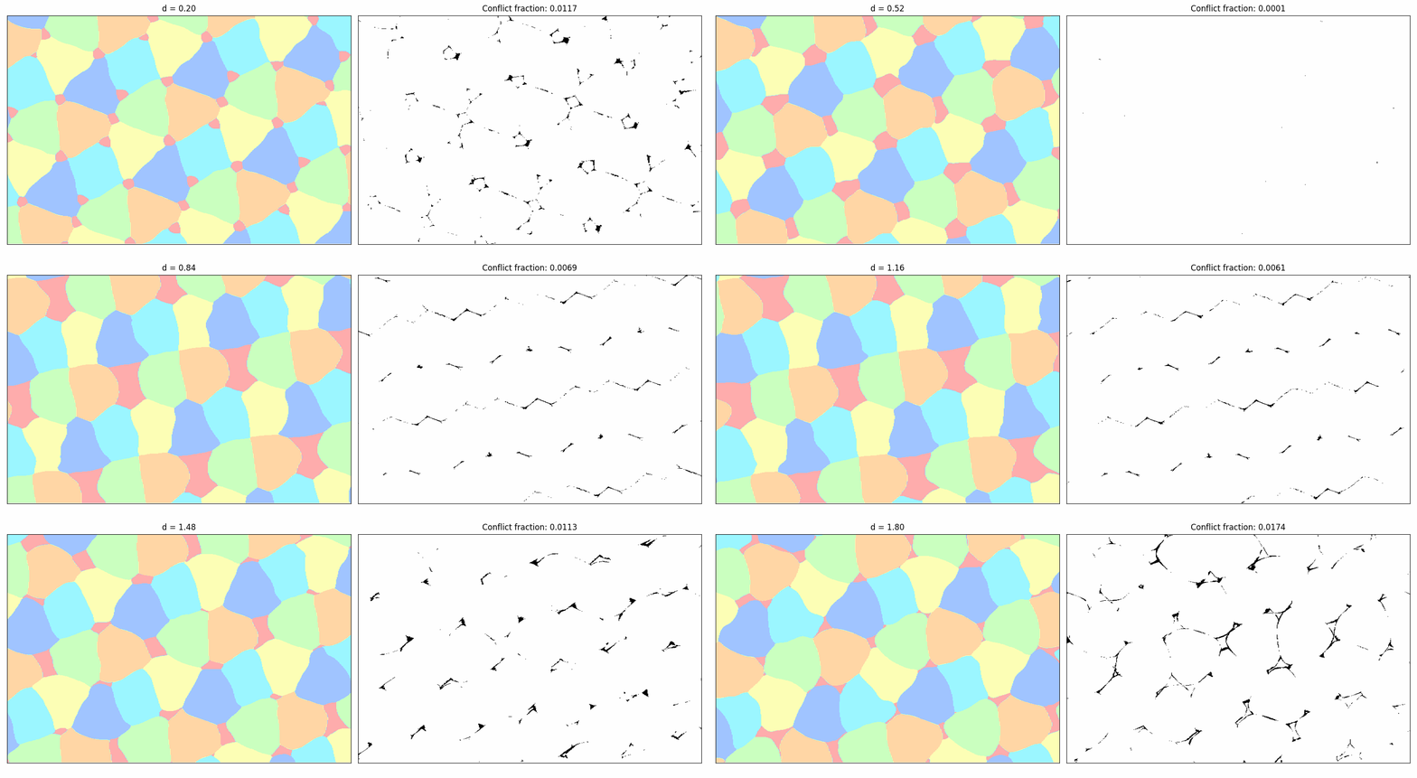
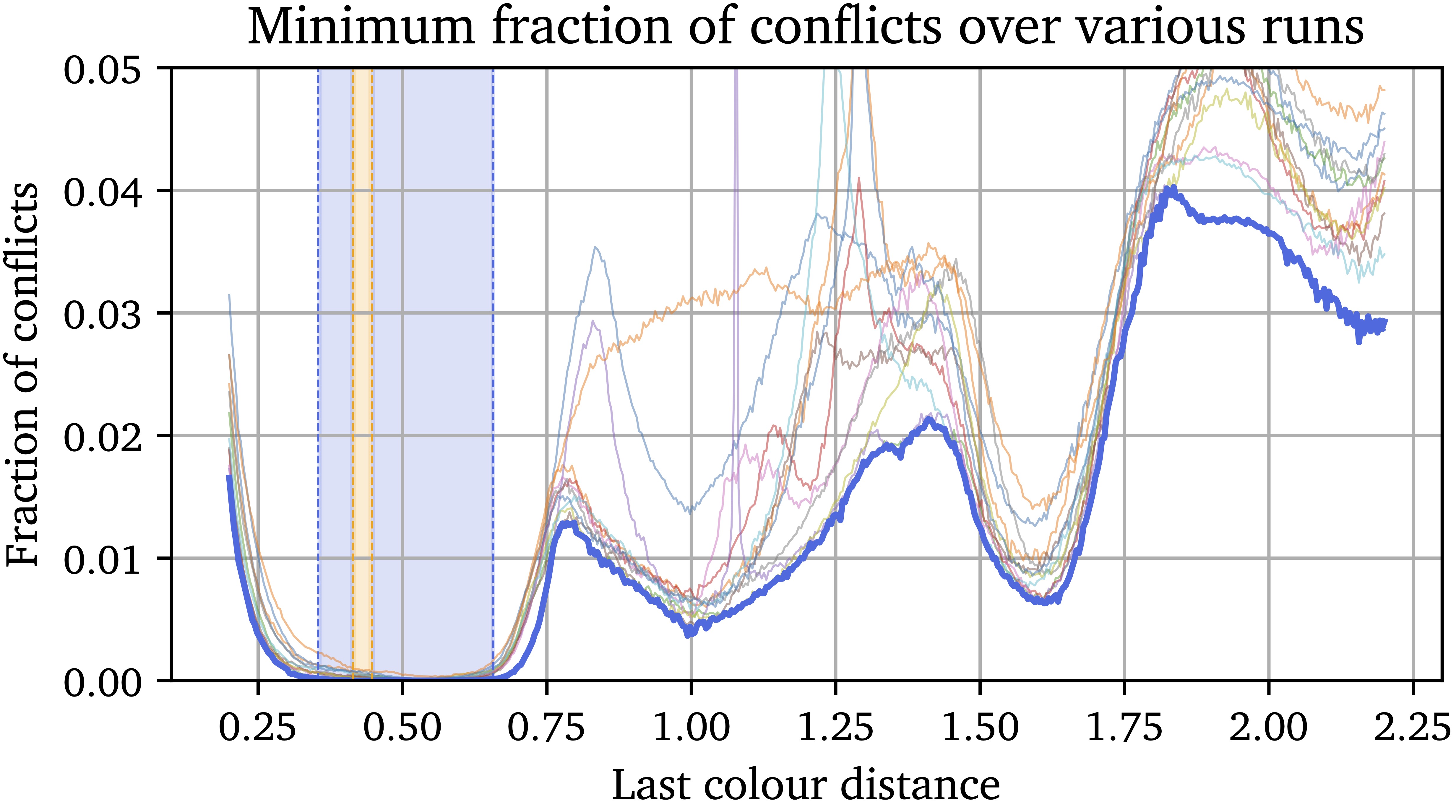
  title={Neural Discovery in Mathematics: Do Machines Dream of Colored Planes?},
  author={Mundinger, Konrad and Zimmer, Max and Kiem, Aldo and Spiegel, Christoph and Pokutta, Sebastian},
  booktitle={Forty-second International Conference on Machine Learning},
  year={2025},
  url={https://openreview.net/forum?id=7Tp9zjP9At},
}</pre> </div>]]></content><author><name>Konrad Mundinger</name></author><category term="deep-learning"/><category term="ai4science"/><category term="ai4math"/><summary type="html"><![CDATA[Our ICML 2025 Oral Paper Neural Discovery in Mathematics: Do Machines Dream of Colored Planes? introduces a novel neural network approach to tackle the famous Hadwiger-Nelson problem and related geometric coloring challenges. We reformulate the combinatorial task as a continuous optimization problem, enabling neural networks to find probabilistic colorings. This led to discovering two new 6-colorings, marking the first progress in 30 years on a key variant involving different forbidden distances and significantly expanding the known solution range.]]></summary></entry><entry><title type="html">Capturing Temporal Dynamics in Tree Canopy Height</title><link href="https://maxzimmer.org/blog/2025/capturing-temporal-dynamics-in-tree-canopy-height/" rel="alternate" type="text/html" title="Capturing Temporal Dynamics in Tree Canopy Height"/><published>2025-05-01T00:00:00+00:00</published><updated>2025-05-01T00:00:00+00:00</updated><id>https://maxzimmer.org/blog/2025/capturing-temporal-dynamics-in-tree-canopy-height</id><content type="html" xml:base="https://maxzimmer.org/blog/2025/capturing-temporal-dynamics-in-tree-canopy-height/"><![CDATA[<div class="series-nav"> <div class="series-header"> <div class="title-row"> <span class="part-badge">Part 2 of 2</span> <h3>Series: Tree Canopy Height Estimation</h3> </div> <p>This post is part of a series of posts on tree canopy height estimation using deep learning and satellite data.</p> </div> <div class="posts"> <a href="/blog/2025/estimating-canopy-height-at-scale/" class="post inactive"> <div class="post-content"> <span class="post-title">Part 1. Global-Scale Forest Height Estimation</span> <span class="post-description">Introduction of the problem of estimating tree height from satellite data, its challenges and how we have overcome them in our ICML24 paper.</span> </div> </a> <div class="post"> <div class="post-content"> <strong class="post-title current">Part 2. Capturing Temporal Dynamics in Canopy Height</strong> <span class="post-description">Part 2 reveals how we moved beyond a single-year map to track changes in canopy height over time, as detailed in our ICML25 paper.</span> </div> </div> </div> </div> <h2 data-nav="Recap">Recap: Learning Forest Height at Scale</h2> <p>This is the second part of the series on <em>Tree Canopy Height Estimation</em>. In <a href="/blog/2025/estimating-canopy-height-at-scale/">Part 1</a>, we discussed the motivation for using deep learning techniques on satellite data for forest height estimation and the challenges involved. We have seen how our method overcomes key technical challenges to generate accurate, high-resolution canopy height maps, resulting in a global forest height map for the year 2020. This post extends that work in an important new direction: we now track the canopy height over time.</p> <h2 id="what-are-we-missing">What Are We Missing?</h2> <p>While having a global forest height map might suggest that no more work is to be done, we are in fact missing out on a lot of information. In this post, we will explore some of the limitations of our current approach and discuss directions for improvements (and, unsurprisingly, how we successfully address them). Two significant issues become apparent:</p> <h3 id="1-tall-trees-are-underpredicted">1. Tall trees are underpredicted.</h3> <p>Current models often struggle to accurately predict the height of tall trees. There’s a consistent underestimation that worsens as the trees get taller. This is a big issue because large trees store most of the carbon, making their accurate prediction crucial for climate analysis.</p> <h3 id="2-maps-only-capture-a-single-year">2. Maps only capture a single year.</h3> <p>Most maps, including our previous work, only capture a single moment in time. However, forests change due to disturbances, logging, and regrowth. Without tracking these changes, we miss the complete picture and can’t fully understand forest history or make informed predictions for the future.</p> <p>Before we discuss how we tackle these challenges, check out the figure below from our paper. It’s a short teaser of how much better we have gotten at predicting tall trees, comparing our latest work with the previous best and ALS data, which we aim to match.</p> <div class="figure-container"> <img src="/assets/img/blog_img/capturing-temporal-dynamics-in-tree-canopy-height/big_trees.jpeg" alt="Performance comparison on tall trees" style="max-width: 100%;" class="zoomable" data-zoomable=""/> <div class="figure-caption">Comparison of six canopy height maps with precise measurements obtained via aerial laser scanning (ALS). The patches contain tall trees exceeding 30 m in height. Our model is the only one that can accurately estimate the height of such trees.</div> </div> <h2 id="addressing-the-challenges">Addressing the Challenges</h2> <p>With these two problems in mind, we aimed to enhance the model from our previous work <d-cite key="paulsestimating"></d-cite>.</p> <p>Regarding the challenge of estimating tall trees, we identified a flaw in almost all existing models: they are trained on composite images, which are aggregations of all images captured over a year. In our previous work, we used the median of images taken at different times. This approach results in a loss of valuable information. We observed that Sentinel-2 images are not perfectly geolocated, and using images from different times allows the model to exploit these minor geolocation errors. Since the satellite does not fly over the exact same spot each time, each 10m pixel captures a slightly shifted reflection of the ground.</p> <p>As a solution, we change our model architecture to a 3D U-Net<d-cite key="cciccek20163d"></d-cite>, which is able to process a stack of monthly images. The monthly data is advantageous, as the model can see variations in structure and pixel reflectance values between seasons and also sees shadows for different sun angles. We modify the model to have a more efficient backbone, as we want to strike a balance between performance and compute needed for large-scale application.</p> <p>We further train not only on image and label for a single year, but from all images and labels from 2019 to 2022 (all years with full GEDI coverage). This way our model becomes invariant to different year-specific color variations and we can apply it to multiple years to get a temporal change map.</p> <h2 id="our-results">Our results</h2> <p>Since we do not preprocess our data to create composite images, the datasets we use are twelve times larger than in our previous work. In consequence, we limit our training and analysis to the European continent, comparing the following maps restricted to this region: Tolan et al. (2023) <d-cite key="tolan2023"></d-cite>, Liu et al. (2023) <d-cite key="liu2023"></d-cite>, Lang et al. (2022) <d-cite key="langGlobalCanopyHeight2022"></d-cite>, Turubanova et al. (2024) <d-cite key="turubanova_europe"></d-cite>, and our previous work Pauls et al. (2024) <d-cite key="paulsestimating"></d-cite>.</p> <div class="table-container"> <table> <thead> <tr> <th>Map</th> <th>Source</th> <th>MAE [m]</th> <th>MSE [m²]</th> <th>RMSE [m]</th> </tr> </thead> <tbody> <tr> <td>Tolan et al. (2023)</td> <td>Maxar</td> <td>11.25</td> <td>212.14</td> <td>13.25</td> </tr> <tr> <td>Liu et al. (2023)</td> <td>Planet</td> <td>8.17</td> <td>138.25</td> <td>10.36</td> </tr> <tr> <td>Lang et al. (2022)</td> <td>S2</td> <td>5.74</td> <td>84.68</td> <td>7.57</td> </tr> <tr> <td>Pauls et al.</td> <td>S1/2</td> <td>5.46</td> <td>83.14</td> <td>7.40</td> </tr> <tr> <td>Turubanova et al.</td> <td>Landsat</td> <td>12.39</td> <td>252.57</td> <td>14.14</td> </tr> <tr> <td><strong>Ours</strong></td> <td><strong>S1/2</strong></td> <td><strong>4.76</strong></td> <td><strong>74.28</strong></td> <td><strong>6.75</strong></td> </tr> </tbody> </table> <div class="table-caption">Despite the coarser 10 m resolution of Sentinel-1/2 (S1/2) compared to Planet (3 m) and Maxar (60 cm), our model yields highly accurate maps and achieves the best overall performance.</div> </div> <p>Our novel approach contributes in three key areas:</p> <h3 id="contribution-1-we-obtain-a-new-state-of-the-art-2020-height-map-for-europe">Contribution 1: We obtain a new state-of-the-art 2020 Height Map for Europe.</h3> <p>Our model outperforms all previous models in both quantitative and qualitative assessments. Compared to the second-best model, we achieve improvements of 13% in MAE, 11% in MSE, and 9% in RMSE. Additionally, our approach provides enhanced forest structure representation, more precisely aligned edges, and better differentiation between forest patches of varying heights.</p> <div class="figure-container"> <img src="/assets/img/blog_img/capturing-temporal-dynamics-in-tree-canopy-height/2020_comparison.jpeg" alt="Qualitative comparison of canopy height maps for the reference year 2020" style="max-width: 100%;" class="zoomable" data-zoomable=""/> <div class="figure-caption">Qualitative comparison of canopy height maps for the reference year 2020.</div> </div> <h3 id="contribution-2-we-obtain-significantly-better-results-for-tall-trees">Contribution 2: We obtain significantly better results for tall trees.</h3> <p>Our model predicts the height of large trees more accurately and is also able to detect single large trees close to larger areas of small trees, which has not been possible before. Further, our approach more closely matches the distribution of the labels and reduces the width of the scatterplot. This improves carbon stock estimates and helps spot old-growth forests.</p> <div class="figure-container"> <img src="/assets/img/blog_img/capturing-temporal-dynamics-in-tree-canopy-height/error_height_distribution.jpeg" alt="Canopy Height Error Distribution" style="max-width: 100%;" class="zoomable" data-zoomable=""/> <div class="figure-caption"> Boxplots for each model showing the 2020 mean error in every 5m bin between 10m and 40m. Although Liu et al. (2023), Pauls et al. (2024) and Lang et al. (2023) perform well on smaller trees, our model performs especially well for taller trees.</div> </div> <div class="figure-container"> <img src="/assets/img/blog_img/capturing-temporal-dynamics-in-tree-canopy-height/combined_scatter_histo_plots.jpeg" alt="Canopy HeightScatterplots and Histograms" style="max-width: 100%;" class="zoomable" data-zoomable=""/> <div class="figure-caption">Left: Scatterplots between 2020 GEDI labels and prediction for different models, including $R^2$ for all labels and $R^2_7$ for labels exceeding 7m. Right: Histograms of GEDI labels and all maps. Turubanova et al. and Tolan et al. saturate at 28 m, our model is the only one matching above 40 m.</div> </div> <h3 id="contribution-3-we-can-track-changes-over-time">Contribution 3: We can track changes over time.</h3> <p>By applying our model across multiple years (2019-2022), we can observe how forests evolve over time. Our approach successfully identifies disturbances and regrowth. However, a four-year span is insufficient to capture very slow growth due to high uncertainty levels.</p> <div class="figure-container"> <img src="/assets/img/blog_img/capturing-temporal-dynamics-in-tree-canopy-height/deforestation.jpeg" alt="TBD" style="max-width: 100%;" class="zoomable" data-zoomable=""/> <div class="figure-caption">Temporal maps illustrate the expansion of deforestation from 2019 to 2022. This is observed by comparing differences between each year, visible in both solitary forest patches surrounded by open land and within densely forested areas.</div> </div> <h2 id="conclusion">Conclusion</h2> <p>Our approach to large-scale temporal forest height estimation surpasses all previous methods in accuracy, particularly for tall trees. Additionally, by applying our model across multiple years, we have developed a temporal change map capable of tracking disturbances and regrowth.</p> <p>A central limitation of our work is that, due to the huge dataset size, we only applied our model to the European continent. We plan to extend our work to the entire world in the future.</p> <p>If you find this work useful, please consider citing our paper:</p> <div class="citation-box"> <div class="citation-header"> <span>BibTeX</span> <button class="bibtex-copy-btn" onclick="copyBibtex()"><span id="copy-text">Copy</span></button> </div> <pre id="bibtex-content">@inproceedings{pauls2025capturing,
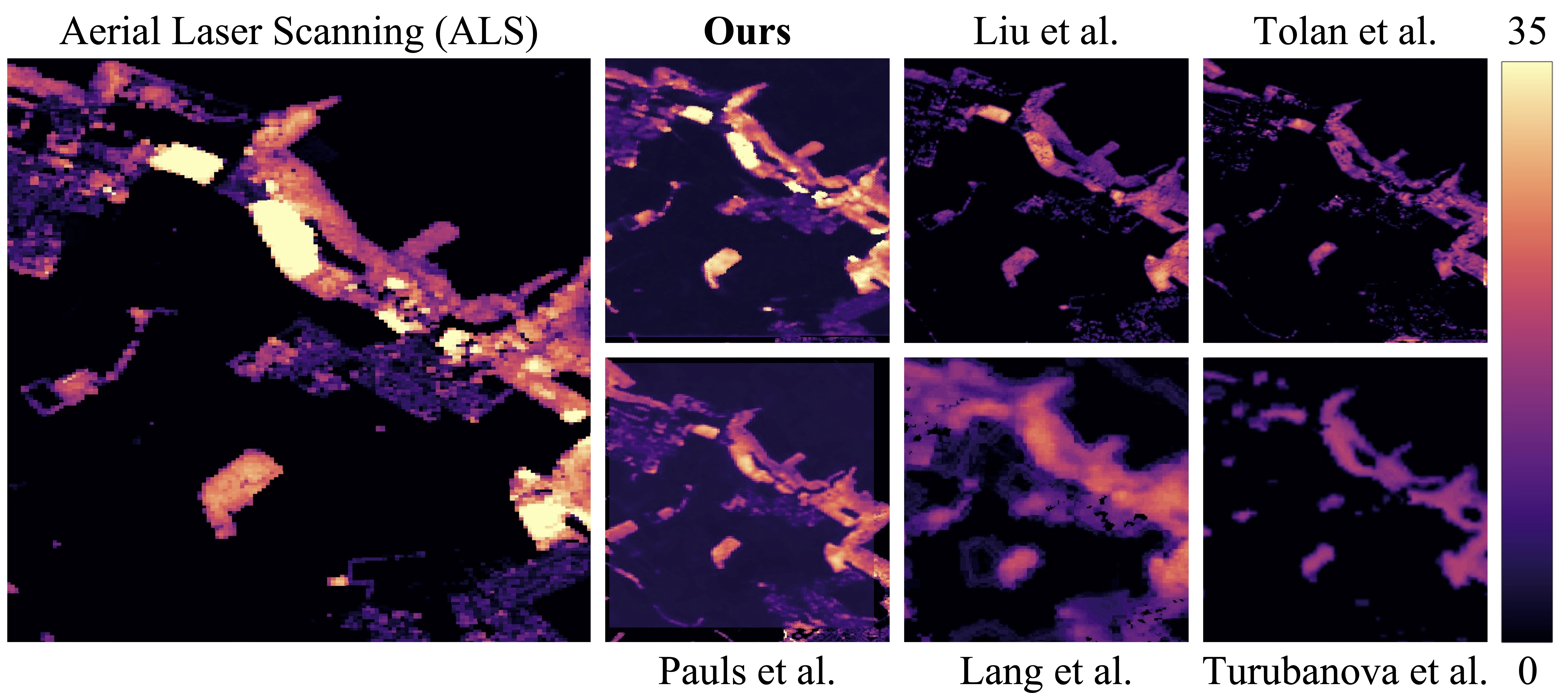
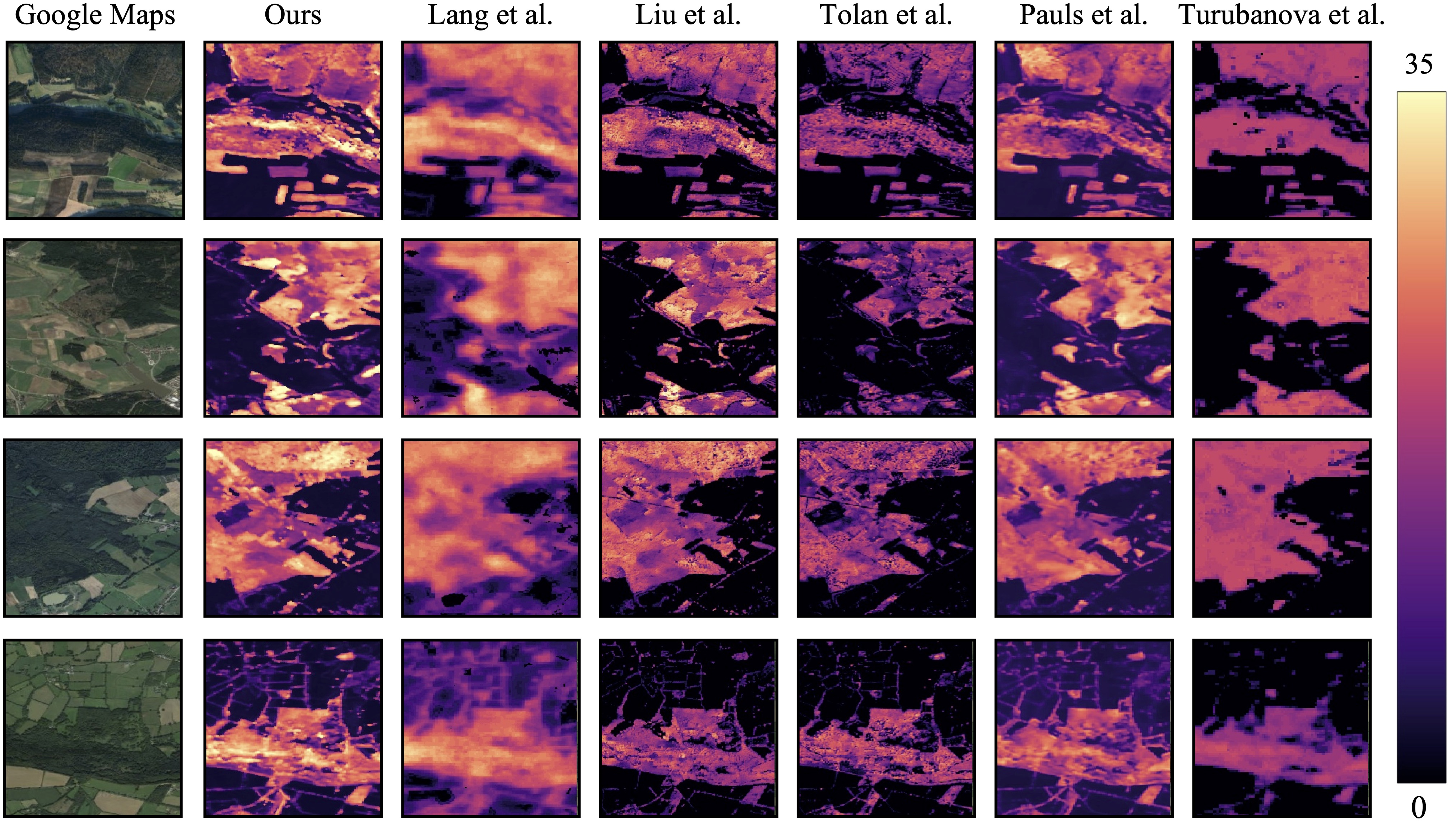
  title={Capturing Temporal Dynamics in Large-Scale Canopy Tree Height Estimation},
  author={Pauls, Jan and Zimmer, Max and Turan, Berkant and Saatchi, Sassan and Ciais, Philippe and Pokutta, Sebastian and Gieseke, Fabian},
  booktitle={Forty-second International Conference on Machine Learning},
  year={2025},
  url={https://openreview.net/forum?id=ri1cs3vtXX}
}</pre> </div>]]></content><author><name>Jan Pauls</name></author><category term="deep-learning"/><category term="ai4science"/><category term="sustainability"/><summary type="html"><![CDATA[Our paper Capturing Temporal Dynamics in Large-Scale Canopy Tree Height Estimation was accepted to ICML 2025! In this work, we present a novel approach to generate large-scale, high-resolution canopy height maps over time. Using Sentinel-2 time series satellite data and GEDI LiDAR data as ground truth, we present the first 10m resolution temporal canopy height map of the European continent for the period 2019-2022. Our pipeline and the resulting temporal height map are publicly available, enabling comprehensive large-scale monitoring of forests.]]></summary></entry><entry><title type="html">Global-Scale Forest Height Estimation</title><link href="https://maxzimmer.org/blog/2025/estimating-canopy-height-at-scale/" rel="alternate" type="text/html" title="Global-Scale Forest Height Estimation"/><published>2025-04-13T00:00:00+00:00</published><updated>2025-04-13T00:00:00+00:00</updated><id>https://maxzimmer.org/blog/2025/estimating-canopy-height-at-scale</id><content type="html" xml:base="https://maxzimmer.org/blog/2025/estimating-canopy-height-at-scale/"><![CDATA[<div class="series-nav"> <div class="series-header"> <div class="title-row"> <span class="part-badge">Part 1 of 2</span> <h3>Series: Tree Canopy Height Estimation</h3> </div> <p>This post is part of a series of posts on tree canopy height estimation using deep learning and satellite data.</p> </div> <div class="posts"> <div class="post"> <div class="post-content"> <strong class="post-title current">Part 1. Global-Scale Forest Height Estimation</strong> <span class="post-description">Introduction of the problem of estimating tree height from satellite data, its challenges and how we have overcome them in our ICML24 paper.</span> </div> </div> <a href="/blog/2025/capturing-temporal-dynamics-in-tree-canopy-height/" class="post inactive"> <div class="post-content"> <span class="post-title">Part 2. Capturing Temporal Dynamics in Canopy Height</span> <span class="post-description">Part 2 reveals how we moved beyond a single-year map to track changes in canopy height over time, as detailed in our ICML25 paper.</span> </div> </a> </div> </div> <h2 id="intro-why-forest-monitoring-matters">Intro: Why Forest Monitoring Matters</h2> <p>Knowing the health and structure of forests is essential for combating climate change. Forests act as a natural carbon sink, absorbing around half of the $CO_2$ from human activities, while also providing habitat for countless species. Yet traditional forest monitoring relies on field workers manually measuring individual trees, an approach that is highly accurate but impractical at global scale. How can we monitor ecosystems that cover nearly one-third of the Earth’s land?</p> <div class="figure-container"> <img src="/assets/img/blog_img/estimating-canopy-height-at-scale/global_big.png" alt="Global canopy height map showing forest heights across the world" style="max-width: 100%;" class="zoomable" data-zoomable=""/> <div class="figure-caption">Our new global canopy height map shows forest heights across the world, with colors indicating tree heights from 0m (black/purple) to 35m+ (yellow).</div> </div> <p>Accurate forest height maps allow scientists to understand how much carbon forests store and how it is distributed, to identify and protect old-growth forests, and to make informed decisions about conservation. The method presented here provides more precise height estimates than previous maps, especially for short vegetation and complex forest areas, enhancing the ability of scientists and policymakers to understand and protect forest resources.</p> <h2 data-nav="The Challenge">The Challenge of Global Forest Monitoring</h2> <p>Traditional forest monitoring through manual measurement of individual trees provides highly accurate data, but it clearly becomes impractical when trying to assess forests at a large scale. Furthermore, there’s a stark divide in monitoring capabilities: industrialized nations often have sufficient resources to conduct comprehensive forest surveys, while many others lack the necessary resources to perform extensive monitoring of their forest landscapes.</p> <p>Satellite technology offers a way forward. Modern satellites can regularly observe the entire Earth, offering a consistent way to monitor forests and general vegetation ecosystems worldwide. In particular, the GEDI mission, which is a full-waveform laser system on the International Space Station, can measure the height of every tree on the surface of the Earth. In practice however, the GEDI measurements are sparsely-distributed, taking up only a tiny fraction of the Earth’s total surface area. This is visible in the image below, where the GEDI measurements are shown in red/yellow dots.</p> <div class="figure-container"> <img src="/assets/img/blog_img/estimating-canopy-height-at-scale/Sentinel_GEDI.jpg" alt="Satellite imagery with height measurements" style="max-width: 100%;" class="zoomable" data-zoomable=""/> <div class="figure-caption">Satellite image overlaid with actual tree height measurements (red/yellow dots) from NASA's GEDI laser system. As the GEDI system is onboard the ISS, you can clearly see the ISS flight paths in the image.</div> </div> <p>The sparse distribution of GEDI measurements poses a fundamental challenge for creating a global map of forest heights. This is where deep learning comes into play. We introduce a methodology to create a <strong>detailed, global-scale map of forest heights</strong> using supervised deep learning on satellite data, combining:</p> <ul> <li>Radar images that can see through clouds (Sentinel-1) as input</li> <li>Optical images that show forest detail (Sentinel-2) as input</li> <li>Height measurements from NASA’s GEDI laser system as ground truth labels</li> </ul> <p>In other words, we train a model that takes satellite images as input and predicts the height of each pixel, training on the sparse GEDI measurements as ground truth labels. But learning heights from satellite images is not easy. Problems like clouds, mountains, and measurement angles make it challenging to get a good estimate of the height of the trees. We discuss our main challenges below:</p> <h3 id="challenge-1-dealing-with-clouds">Challenge 1: Dealing with Clouds</h3> <p>Satellites follow fixed orbits and capture images on a regular schedule, regardless of cloud cover. While most regions experience clear skies at some point during the year, allowing us to select cloud-free images, tropical regions pose a unique challenge. The persistent cloud cover and high-altitude cirrus clouds in these areas make it difficult to obtain clear optical satellite imagery, necessitating innovative approaches to extract useful data.</p> <h3 id="challenge-2-mountains-and-measurements">Challenge 2: Mountains and Measurements</h3> <div class="figure-container"> <img src="/assets/img/blog_img/estimating-canopy-height-at-scale/CanopyProblem.png" alt="The challenge of measuring trees on slopes" style="max-width: 100%;" class="zoomable" data-zoomable=""/> <div class="figure-caption">How slopes affect height measurements: the same tree might appear taller when measured on a slope, and even in the absence of trees, GEDI records a height measurement due to the elevation change within its footprint.</div> </div> <p>Mountainous terrain poses unique measurement challenges. GEDI’s laser technology measures the height difference between the highest and lowest points within a 25-meter diameter circle. On steep slopes, this can distort measurements in two ways: trees may appear artificially taller than their true height, and even bare slopes register as having “height” due to the elevation change within the measurement circle.</p> <h3 id="challenge-3-location-accuracy">Challenge 3: Location Accuracy</h3> <div class="figure-container"> <img src="/assets/img/blog_img/estimating-canopy-height-at-scale/gedi_shift.png" alt="Shifted measurements example" style="max-width: 100%;" class="zoomable" data-zoomable=""/> <div class="figure-caption">GEDI measurements can be slightly offset from their true location due to GPS and positioning errors (each circle shows a height measurement).</div> </div> <p>Even with accurate height measurements, GPS and satellite positioning errors can cause misalignment between reported and actual measurement locations. This spatial offset presents a critical challenge: how can we train a reliable model when the ground-truth data may be shifted from its true position?</p> <h2 data-nav="Our Approach">Our Approach to Forest Height Estimation</h2> <div class="figure-container"> <img src="/assets/img/blog_img/estimating-canopy-height-at-scale/pipeline.png" alt="Our processing pipeline" style="max-width: 100%;" class="zoomable" data-zoomable=""/> <div class="figure-caption">Overview of our approach: from satellite data to the global height map.</div> </div> <p>The solution involves three main components:</p> <p>(1) <strong>Multiple Types of Satellite Data</strong></p> <p>Our approach leverages two complementary satellite data sources from ESA: Sentinel-2’s high-resolution optical imagery (similar to Google Maps) and Sentinel-1’s radar data. The radar signals can penetrate clouds and even some vegetation layers, providing crucial data in areas where optical sensors are limited. We combine these inputs with height measurements from NASA’s GEDI laser system on the International Space Station, which serve as our ground truth labels.</p> <p>(2) <strong>Smart Cloud Handling</strong></p> <p>Although we use radar data, it is still beneficial to use optical data as often as possible, as it has a higher level of detail. We therefore try to construct a cloud-free image where possible. Sentinel-2 does not only capture a single image per year, but an image of the entire globe every 6 days. We therefore make use of all images and mask out clouds from every image. Lastly, we combine all images into a single image by taking the per-pixel median of all non-cloud pixel values. This step effectively removes almost all clouds from the image and reduced noise and inter-year-variability.</p> <p>(3) <strong>Model Training</strong></p> <p>We used a special loss function to address location erros in our ground-truth measurements. Our loss function allows the model to shift the measurements within a certain range if it is similar for all nearby measurements. Secondly, we pre-filter our labels to remove measurements that were taken on areas with a great slope.</p> <h3 id="results-comparing-to-existing-maps">Results: Comparing to existing maps</h3> <div class="figure-container"> <img src="/assets/img/blog_img/estimating-canopy-height-at-scale/global_and_regional_comparison.png" alt="Comparison of different approaches" style="max-width: 100%;" class="zoomable" data-zoomable=""/> <div class="figure-caption">Comparison of our map (second row) with previous global maps and a detailed regional map (our benchmark). Notice the improved detail in our results.</div> </div> <p>Visually, our new method shows significant improvements over existing global maps, successfully surpassing their accuracy and detail levels. Specifically, we achieve better detail in forest structure, more accurate height estimates, and clearer distinction between forest and non-forest areas. The visual quality of our results even closely approaches that of specialized regional maps.</p> <p>Let’s look at how well our method performs quantitatively. We compared our results with the two other existing global canopy height maps, namely the one from Lang et al. <d-cite key="langHighresolutionCanopyHeight2023"></d-cite> and the one from Potapov et al. <d-cite key="potapovMappingGlobalForest2021"></d-cite>, reporting metrics for all ground-truth measurements as well as only for ground-truth measurements with a height greater than 5m to emphasize the error on trees.</p> <div class="table-container"> <table> <thead> <tr> <th>Method</th> <th>Mean Absolute Error</th> <th>Root Mean Square Error</th> <th>Mean Absolute Error (for labels &gt; 5m)</th> <th>Root Mean Square Error (for labels &gt; 5m)</th> </tr> </thead> <tbody> <tr> <td>Lang et al.</td> <td>6.47m</td> <td>8.62m</td> <td>8.80m</td> <td>11.02m</td> </tr> <tr> <td>Potapov et al.</td> <td>6.92m</td> <td>9.25m</td> <td>10.01m</td> <td>12.43m</td> </tr> <tr> <td><strong>Our Method</strong></td> <td><strong>2.43m</strong></td> <td><strong>4.73m</strong></td> <td><strong>4.45m</strong></td> <td><strong>6.72m</strong></td> </tr> </tbody> </table> <div class="table-caption">Performance comparison of different canopy height estimation methods.</div> </div> <p><em>Our method achieves significantly lower errors across all metrics. For trees taller than 5m, we maintain this advantage with a mean absolute error of just 4.45m.</em> To better understand where our method performs well and where there’s still room for improvement, let’s look at the error distribution across different tree heights:</p> <div class="figure-container"> <img src="/assets/img/blog_img/estimating-canopy-height-at-scale/error_height_distribution.png" alt="Error distribution across tree heights" style="max-width: 100%;" class="zoomable" data-zoomable=""/> <div class="figure-caption">Error analysis across different height ranges. The boxes show the distribution of errors for each height range, with negative errors indicating underestimation. Notice how we (blue) maintain lower error rates and less variance, especially for trees up to 30m.</div> </div> <p>Looking at this analysis in detail, our method shows excellent performance for trees up to 20m in height, with strong accuracy continuing through the medium height ranges. However, we must acknowledge that very tall trees, particularly those above 30m, remain a significant challenge. This is especially pronounced in tropical forests, where canopy heights can exceed 40m - an important area we need to address in future work. Nevertheless, even with these challenges in tall tree estimation, our approach demonstrates notably lower error variance compared to previous methods across most height ranges.</p> <h2 id="conclusion">Conclusion</h2> <p>Creating accurate global forest height maps is crucial for understanding and protecting our planet’s forests. Our method combines the latest satellite technology with machine learning to produce the most detailed and accurate global forest height map to date. While we’ve made significant progress, there’s still more to explore. Future improvements could include:</p> <ul> <li>Even better handling of mountainous regions</li> <li>More frequent updates to track changes over time</li> <li>Reducing the error for very tall trees</li> </ul> <p>Want to explore forest heights in your area? Our global canopy height map is available on Google Earth Engine. You can view our predicted forest height information for any location on Earth here: <a href="https://worldwidemap.projects.earthengine.app/view/canopy-height-2020">worldwidemap.projects.earthengine.app/view/canopy-height-2020</a>.</p> <p>If you find this work useful, please consider citing our paper:</p> <div class="citation-box"> <div class="citation-header"> <span>BibTeX</span> <button class="bibtex-copy-btn" onclick="copyBibtex()"><span id="copy-text">Copy</span></button> </div> <pre id="bibtex-content">@inproceedings{pauls2024estimating,
  title={Estimating Canopy Height at Scale},
  author={Jan Pauls and Max Zimmer and Una M. Kelly and Martin Schwartz and Sassan Saatchi and Philippe Ciais and Sebastian Pokutta and Martin Brandt and Fabian Gieseke},
  booktitle={Forty-first International Conference on Machine Learning},
  year={2024},
  url={https://openreview.net/forum?id=ZzCY0fRver}
}</pre> </div>]]></content><author><name>Jan Pauls</name></author><category term="deep-learning"/><category term="ai4science"/><category term="sustainability"/><summary type="html"><![CDATA[Our paper Estimating Canopy Height at Scale was accepted to ICML 2024! In this work, we present a novel framework for global-scale forest height estimation. Using a deep learning approach that leverages large amounts of satellite data with only sparsely distributed ground-truth height measurements from NASA's GEDI mission, we achieve state-of-the-art accuracy with MAE/RMSE of 2.43m/4.73m overall, significantly outperforming existing approaches. The resulting height map facilitates ecological analyses at a global scale.]]></summary></entry></feed>